Schema-As-You-Go: On Probabilistic Tagging and Querying of Wide Tables Meiyu Lu‡
Divyakant Agrawal§
Bing Tian Dai‡
School of Computing National University of Singapore
Department of Computer Science University of California, Santa Barbara
{lumeiyu, dbt, atung}@comp.nus.edu.sg
[email protected]
ABSTRACT The emergence of Web 2.0 has resulted in a huge amount of heterogeneous data that are contributed by a large number of users, engendering new challenges for data management and query processing. Given that the data are unified from various sources and accessed by numerous users, providing users with a unified mediated schema as data integration is insufficient. On one hand, a deterministic mediated schema restricts users’ freedom to express queries in their preferred vocabulary; on the other hand, it is not realistic for users to remember the numerous attribute names that arise from integrating various data sources. As such, a user-oriented data management and query interface is required. In this paper, we propose an out-of-the-box approach that separates users’ actions from database operations. This separating layer deals with the challenges from a semantic perspective. It interprets the semantics of each data value through tags that are provided by users, and then inserts the value into the database together with these tags. When querying the database, this layer also serves as a platform for retrieving data by interpreting the semantics of the queried tags from the users. Experiments are conducted to illustrate both the effectiveness and efficiency of our approach.
Categories and Subject Descriptors H.2.8 [Database Management]: Database applications
General Terms Management, Performance
Keywords Probabilistic Tagging, Wide Table, Top-k Query Processing
1.
Anthony K.H. Tung‡
§
‡
INTRODUCTION
The rapid growth of Web 2.0 technologies and social networks has provided us with new opportunities for sharing
Permission to make digital or hard copies of all or part of this work for personal or classroom use is granted without fee provided that copies are not made or distributed for profit or commercial advantage and that copies bear this notice and the full citation on the first page. To copy otherwise, to republish, to post on servers or to redistribute to lists, requires prior specific permission and/or a fee. SIGMOD’11, June 12–16, 2011, Athens, Greece. Copyright 2011 ACM 978-1-4503-0661-4/11/06 ...$10.00.
data and collaborating with others. Within a community, users may like to contribute their own data, share the data with friends, and meanwhile explore the shared data at the community scale. Effectively and efficiently managing and exploring these data at a web-scale level is an interesting and important problem. In this paper, we focus on the management of shared structured tables (e.g. Google fusion table [16]) which is an important type of data in Web 2.0. Such data have some inherent properties that make their management challenging. Heterogeneity. Data provided by different users may be widely heterogeneous, containing different attribute names that describe semantically similar values or same attribute name with different semantics. For example, in Figure 1(a), user A chooses attribute make to describe the car manufacturer in his/her private data, while user B uses manufacturer to represent the same meaning. Similarly, the semantics of car in (b) is model but in (c) it contains both make and model information. Numerosity. As all users can publish their data into the community as shown in Figure 1(a), (b) and (c), the number of distinct attributes will grow drastically as more users participate. This results in a wide table [7] as Figure 1(d) which is essentially a structured table with a large number of attributes and many empty cells. Given such a wide table, most existing data integration approaches [23] create a global mediated schema that usually contains a huge number of attributes. Such huge mediated schema is difficult to query as users cannot remember all the attributes. Therefore, a more flexible and user-oriented query interface is required. This interface should allow users to choose different attribute names to represent the same semantics in different queries, and have the power to express their confidence over the attribute semantic heterogeneity in posed queries. Personalized Attributes. Since attributes are contributed by users, there could be many personalized attributes, which cannot be captured by existing ontology or taxonomy, such as DBpedia1 and WordNet2 . Examples of such personalized attributes include myear in Figure 1(c), which represents the production year of a car, and eadd, the abbreviation for email address. Due to this, existing techniques that rely on ontology for schema mapping [26, 30] will not be suitable any more. A better system should be able to infer more popular 1 2
DBpedia, http://dbpedia.org/About WordNet, http://wordnet.princeton.edu
User A
make
model
Ford
Fiesta
BMW
318Ci
(a)
make
manufacturer
model
car
myear
T1
Ford
--
Fiesta
--
--
BMW
--
318Ci
--
--
manufacturer
car
Ford
Focus 1.6A
T3
--
Ford
--
Focus 1.6A
--
Accord
T4
--
Honda
--
Accord
--
T5
--
--
--
BMW 525i
2005
T6
--
--
--
Toyota Camry
2009
Honda
(b) car
myear
BMW 525i
(d)
2005
Toyota Camry
Tag1 make make manufacturer model
TID
T2
User B
User C
Q1 Q2
User F Q3 Q4 User G
2009
(c)
Tag2 manufacturer car car car
Figure 1: The Wide Table Similarity 0.95 0.5 0.52 0.65
Figure 2: Tag Similarity attributes for such personalized ones, so that these data can be explored by the other users asides from its owner. Due to the inherent semantic heterogeneity of the attributes in user contributed data, we will no longer refer to them as “attribute”. Instead, we borrow the term tag from the multimedia domain [1, 2], and view these attribute names as just a way to annotate the values that are provided by users3 . In this paper, we describe a query system which enables users to effectively query a large quantity of user contributed data. Our system provides the following functionalities. • Users can contribute and share data by inserting them into a single wide table together with their tags, as shown in Figure 1(d). • Our system is able to automatically discover the semantic relationships between users’ tags, which is handled by our tag inference approach in Section 3. Figure 2 illustrates the semantic similarities between each pair of tags produced by our approach for the example data in Figure 14 . • Users can use their own preferred tags to query the database, and the system then dynamically determines the semantics of these tags at query time. Combining the data from Figure 1(d) with the tag similarities in Figure 2, we can easily obtain the virtual probabilistic tagged data, as shown in Figure 3, where each value is associated with a list of htag, probabilityi pairs. The probability indicates the semantic association strength between the value and tag pair. The generation of such semantic association probabilities is called probabilistic tagging, and its formal definition will be given in Section 2. We next present an example to illustrate several characteristics of our query interface via a set of queries. 3
User E
In this case, users might even choose to annotate the same value with multiple tags. 4 As our similarity measure is symmetric, we only show unidirectional tag similarity in Figure 2.
User H
Example 1. Figure 1 shows a scenario where four users, A, B, C and D contribute and share their datasets. The wide table is used to store the shared data. User E, F, G and H then submit four different queries which are Q1, Q2, Q3 and Q4, respectively. The queries are shown in Table 1 in an extended SQL format. The delimiter ‘ @’ in the query is for users to explicitly specify their confidence over tag semantics. Its formal definition is presented in Section 2. Here we can interpret make @0.9 as a set of tags in Figure 2 which are similar to make with confidence no less than 90%. The table name CAR refers to the probabilistic tagging table in Figure 3. Values in the result tuples have the same order as the tags in the SELECT clause. From the query result in Table 1, we observe that i) different users can choose different tags to express the same semantics, such as Q1 and Q2; ii) explicit confidence specification gives users control over the search scope. For instance, with lower confidence Q3 retrieves two more tuples than Q1; iii) schema for users’ query is dynamically determined at query time, which is user-oriented rather than predefined. Take Q4 as an example, where a user would like to retrieve values that are associated with car and model from CAR. From the data perspective, for T3 and T4, tag car in the query should be aligned with car in the source table. But from the users’ perspective, intuitively the best schema alignment for T3 and T4 should be (car, model). This is what our system retrieves given Q4. To further see the benefit of our approach, Figure 4 shows the result of Q4 over tuples T3 and T4 using our approach and the one proposed by Dong and Halevy in [12, 25]5 . Both records returned by our approach are correct and ranked in the right order. However, the top two ranked tuples retrieved by probabilistic integration are not correct although their score is much higher than the correct ones. The result differs because we are dynamically determining the semantics for user posed tags at query time. The reasons for such differences will be explained in Section 2.2. Besides the functionalities discussed above, our work also makes the following contributions: • We proposed the concept of probabilistic tagging to represent the associations between values and tags. • We presented an effective distance function to measure the semantic distance between a pair of tags. Based 5 Please refer to Appendix A for the detailed score computation for probabilistic integration.
Table 1: Example Queries QID Q1 Q2 Q3 Q4
Query SELECT
[email protected] FROM CAR; SELECT
[email protected] FROM CAR; SELECT
[email protected] FROM CAR; SELECT car, model FROM CAR;
TID
Value
Probabilistic Tagging
T1
Ford
,,
T1
Fiesta
,
T2
BMW
,,
T2
318Ci
,
T3
Ford
,,
T3 T4
Focus 1.6A Honda
,,, ,,
T4 T5
Accord BMW
,,, ,,,
T5
2005
T6
Toyota
,,,
T6
2009
Figure 3: Probabilistic Tagging QID
Q4
Query
SELECT car, model FROM CAR
Our Result
TID T3 T4
car Ford Honda
model Focus 1.6A Accord
rank 1 2
Data Integration Result
TID T3 T4 T3 T4
car Focus 1.6A Accord Ford Honda
model Focus 1.6A Accord Focus 1.6A Accord
rank 1 2 3 4
Figure 4: Query Result Comparison on this, we are able to automatically infer semantically similar tags for each value. • We proposed an efficient dynamic instantiation approach to associate the queried tags and data values during query processing. • A complete and extensive experimental study is conducted to validate our approach.
2.
PROBLEM DEFINITION
2.1 Probabilistic Tagging As discussed earlier, one of our main objectives is to provide a flexible interface, which allows users to query the underlying database with any tag they like. The very first challenge is to discover which tags are similar in semantics. However, this is insufficient since some tags are more similar to each other in semantics while others are not. Taking T1 in Figure 3 as an example, it is intuitive that the semantics of ‘Ford’ is better reflected by manufacturer than car since the semantics of manufacturer is quite specific, while car is
Result T1(Ford),T2(BMW),T3(Ford),T4(Honda) T1(Ford),T2(BMW),T3(Ford),T4(Honda) T1(Ford),T2(BMW),T3(Ford),T4(Honda), T5(BMW 525i),T6(Toyota Camry) T1(Ford,Fiesta),T2(BMW,318Ci), T3(Ford,Focus 1.6A),T4(Honda, Accord)
a relatively more general term. Therefore, the second issue is that the semantic association strength between a value and tag should be well quantified, as shown in Figure 3. In this paper, for a given value v in the wide table, we interpret its semantic association with a tag t as the likelihood/belief that v is tagged by t. Definition 1 (Probabilistic Tagging). Let T be a set of tags, for a value v in Wide Table and a tag t ∈ T , probabilistic tagging refers to the process of associating a probability ζv,t for v and t, such that value v is tagged by tag t with probability ζv,t . The probability ζv,t is called the associated probability or association probability. If the semantic association between value v and tag t is stronger, then their associated probability ζv,t will be higher and vice versa. As shown by T1 in Figure 3, for the value ‘Ford’, its associated probability with its original tag make is 1.0 while its associated probability with inferred tags manufacturer and car are 0.95 and 0.5, showing difference in the strength of semantic association. We note here that unlike previous works [12, 25, 17] in data integration, the probabilities for all tags being associated with a value v do not sum up to 1. This is because there is no assumption of mutual exclusion between tags at this stage of data processing. We avoid doing so to prevent a label bias problem in which a value v will have much lower associated probability with each tag if it can be semantically described by many different tags. For example, a value associated with 5 or more tags will have much lower probability than value with 2 or less tags. Instead, we choose to introduce the assumption of mutual exclusion during query time where the semantic meaning of the tags are clearer.
2.2 Query Semantics After discovering and quantifying the tag semantic relationships during probabilistic tagging, the resulting probabilistic table is shown as in Figure 3. In this table, each value is associated with a htag, probabilityi pair list. Query over such probabilistic table is much more challenging than with a predefined schema. We will now look into the query relevant issues over a probabilistically tagged table.
2.2.1 Extended SQL Query In this paper we adopted a SQL like query syntax to support our tag based queries. Specifically, we extended SQL query to allow users to express their semantic confidence for each tag using the delimiter ‘@’. We show some examples in Table 1. Below is a more complex extended SQL query. SELECT FROM WHERE AND AND
car,
[email protected],
[email protected] CAR
[email protected] = ‘Ford’ price ≥ 10,000 price ≤ 20,000
When a user provides a tag with high confidence, it means that he is very sure about the semantics of the tag, and does not want our system to do much tag inference. In contrast, if the user is unsure of the semantics and he likes to use more tags that are similar to the queried tag, then he can provide a lower confidence threshold. Definition 2 (Tag Expansion). Given a tag tq and its semantic confidence δ in query q, tq @δ refers to the expanded tag set Te = {tei |i = 1, . . . , n}, where for each tag tei ∈ Te , Semsim(tq , tei ) ≥ δ. We call Te as the expanded tag set for tq . In the above definition, Semsim(tq , tei ) is the semantic similarity between tag tq and tei , which is formally defined by Equation 6 in Section 3. When processing query q, tq will be expanded to a tag set Te , a set of tags that are semantically similar to tq based on a threshold δ. All values that are originally associated with any of the tags in Te are valid for this tag expansion condition, and should be taken into consideration when answering the query. If no semantic confidence is explicitly specified for tq , we will expand it to all our inferred tags. Take the queries in Table 1 as example,
[email protected] will be expanded to all the tags that are similar to make in semantics inferred by our system, that is {manufacturer,car}, but
[email protected] will only be expanded to {manufacturer}.
2.2.2 Query Answering Before explaining the semantics of query answering, we first look at the intuitions behind our query answering techniques. Intuitively, syntactically equivalent tags in user posed queries should be instantiated with the same value, no matter how many places it appears in the query. For example, although price occurs three times in the example query in Section 2.2.1, once in the SELECT clause and twice in the WHERE clause, it is obvious that all the occurrences of price refer to exactly the same semantics, i.e. price of a car. Thus, in the resulting record, all these three instances of price should be instantiated with the same value. Based on this, we proposed the following Consolidation Rule for our query answering. Rule 1 (Consolidation Rule). Let set Tq = {ti |i = 1, . . . , n} be the set of tags in query q, for two tags ti , tj ∈ Tq , if ti = tj , then ti and tj should be instantiated with the same value from the underlying record.
argued that car in the query should be aligned with manufacturer in the source table. Here we look at the query in Section 2.2.1, where a user would like to retrieve the value associated with car from a record whose value ‘Ford’ is associated with make (for simplicity, we skipped the other constraints). Now for T3, it is more reasonable for car in the query to be aligned with car in the source table. Comparing these two queries, we can see that with our mutual exclusion rule, the same tag (car) can be aligned with different semantics in different queries even for the same record (T3). As explained earlier, applying the mutual exclusion rule during query answering time allows us to avoid the label bias problem. Moreover, our mutual exclusion rule cannot be trivially introduced in [12, 25, 17] since they enforced the fact that two attributes/tags are either semantically equivalent (associated with the same value) or not in each possible world. As such, the problem illustrated by Figure 4 in Example 1 is inherent for [12, 25, 17]. For a given tuple/record, we aim to find its possible best alignment to the queried tags. As the semantics of queried tags are determined dynamically on the fly, our query answering is referred to as Dynamic Instantiation. Definition 3 (Dynamic Instantiation). Let set Tq = {ti |i = 1, . . . , n} be the set of tags in query q, and Vr = {vj |j = 1, . . . , m} be the set of values from a record r, we refer to a mapping f : Tq → Vr as the dynamic instantiation of Vr with respect to Tq . Based on f , the instantiated score Score(r) for r with respect to q is defined as the multiplication Q of associated probabilities for edges in f , i.e. Score(r) = n i=1 ζf (ti ),ti . In addition, all the following conditions must be satisfied in f : 1. f satisfies all the value constraints in the WHERE clause. 2. f satisfies both Consolidation Rule and Mutual Exclusion Rule; 3. The associated probability for each edge in f , i.e. ζf (ti ),ti , must satisfy its corresponding tag expansion; 4. Among the mappings in which all the above three conditions hold, dynamic instantiation refers to f whose score is maximized, i.e. f = arg maxf Score(r).
Rule 2 (Mutual Exclusion Rule). Let Tq = {ti |i = 1, . . . , n} be the set of tags in query q, for two tags ti , tj ∈ Tq , if ti 6= tj , then ti and tj should be instantiated with different values from the underlying record.
The first condition states that if tag t has value constraints in the WHERE clause, then its mapped value f (t) should satisfy all the value constraints over t in query q. The second condition is for us to better capture the users’ intention as discussed earlier. The third condition is used to meet the tag semantic specifications. Finally, the last condition is to find the best possible instantiation between tags set Tq and values set Vr , i.e. the one with maximum instantiation score Score(r). Our instantiated score is defined as the multiplication of associated probabilities in the instantiation f , that is because in our case the associations between tag and value pairs are independent, and based on our mutual exclusion rule, all the edges falling outside of f are invalid. Due to the semantic uncertainty of tags, answering a query q can result in a large number of records with score larger than 0. In view of this, we mainly focus on top-k query processing to find the best k answers based on our query answering semantics.
We have discussed the impact of our mutual exclusion rule using Q4 earlier (in Example 1). There for T3, we
Definition 4 (Top-k Query Answering). Given a query q, a user specified positive integer k, and a set of
Consider the query in Section 2.2.1, although we know tag car and make are similar in semantics from Figure 2, in this query they actually represent different attributes because the user specifies them as different. In other words, car and make are mutually exclusive from each other in this query, and should be instantiated with different values in the resultant record. We proposed our Mutual Exclusion Rule as below.
records R = {ri |i = 1, . . . , |R|}, the problem of top-k query answering is to retrieve a record set RS, such that RS ⊆ R, |RS| is maximized with the condition |RS| ≤ k, ∀r ∈ RS and ∀r ′ ∈ RS, which is the complementary set of RS, Score(r) ≥ Score(r ′ ). From the above definition, it is possible that less than k results are retrieved. We however feel that it is a worthy cost to pay for freeing users from a fixed mediated schema and providing relaxation over the tag specifications.
3.
TAG INFERENCE
We next describe our tag inference process which is essential for discovering the semantic relationships between tags, and computing the associated probabilities between tag and value pairs. We use T = {ti |i = 1, . . . , n} to denote all the tags in our database, and V = {vj |j = 1, . . . , m} to denote all the values. For a tag t ∈ T , we use Vt ⊆ V to represent the set of values that fall under the tag t in the wide table. Effectively discovering the semantic similarities between user contributed tags however is challenging. Although several approaches have been proposed in the literature [23, 26, 30], none of them is suitable for our case. First, string similarity over tag names could not convey all cases [26, 23]. With such approaches, model and model_year will be treated as similar but make and manufacturer will be treated as dissimilar. Second, ontology and taxonomy based methods [26, 30] are not applicable, as there are many personalized tags like myear and eadd, which cannot be captured by any existing ontology and taxonomy. Finally, similarity function based on values overlap [23] works only for categorical values, not for string and numerical values. For example, given two set of emails that are contributed by different users using two different tags, it is unlikely that there is much overlap between the two set of emails. Our approach to discovering the semantic similarities in this paper can generally be described in two steps. First, soft clustering [28] is applied to the values in the wide table to separate them probabilistically into K clusters, i.e. each value can belong to each of the K clusters with different probabilities. Since each tag is associated with a set of values with different probabilities, we can thus indirectly compute the probability of these tags being associated with the K clusters. In the second step, we measure the distance between tags by comparing the probability distribution of their associated membership to each of the K clusters using KL-divergence [8, 9]. KL-divergence is a function for measuring the relative entropy between two distributions. Specifically, if the probabilistic cluster membership distributions for two tags are pPand q respectively, their relative entropy is KL(pkq) = i=1..K pi log pqii , where pi is the probability of the first tag being associated to cluster i and qi is the probability of the second tag being associated to cluster i.
3.1 Tag Semantic Distance Discovery To perform the soft clustering, our approach first extracts a set of features F from the underlying data V . Depending on the type of values in t, different approaches are adopted to generate the features for t. If values in t are string values, we extract a set of frequent q-grams called sigrams as its features. If values in t are numerical values, bins of the distribution histogram over Vt are extracted as its features.
After extracting the features F for all values V , soft clustering [28, 8] is performed over F. In soft clustering, the membership of a value in a cluster is probabilistic. Suppose there are K clusters C = {c1 , . . . , cK }, for a value v, its membership probabilities P in each cluster form a vector τ (v) = hp1 , . . . , pK i, where K i=1 pi = 1, and pi is the probability that v belongs to cluster ci . We call τ (v) the cluster probability distribution for value v over C. Based on [8], our soft clustering based tag inference is robust when K>100. We set K to be 200 in this paper. Since a tag t can be associated with different values which have different cluster probability distributions on the K clusters, we can indirectly compute a cluster probability distribution for a tag t (denoted as τ (t)) by taking the average cluster probability distributions of all its associated values Vt : X 1 · τ (vt ) τ (t) = |Vt | v ∈V t
t
To measure the semantic relationship between two tags, t1 and t2 , one important factor that needs to be considered first is the semantic scope of each of these tags. Intuitively, if the semantics of a tag t is more general, the values associated with it will be more diverse. For instance, both make and model information of a car can be tagged by car, while only the make information can be tagged by make. Thus, the semantic scope Scope(t) for tag t can be captured by the average KL-divergence between τ (vt ) and τ (t): X 1 Scope(t) = · KL(τ (vt )||τ (t)) (1) |Vt | v ∈V t
t
Another important factor we need to consider is the distance between tag t1 and the values of tag t2 . If t1 is similar to t2 , then τ (vt1 ) should be close to τ (t2 ). For clarity, we define the distance between the value set Vt1 of tag t1 and another tag t2 as DV (Vt1 , t2 ): X 1 DV (Vt1 , t2 ) = (2) · KL(τ (vt1 )||τ (t2 )) |V t1 | v ∈V t1
t1
Based on the above discussion, if two tags t1 and t2 are similar in semantics, they should i) have similar semantic scopes; and ii) close to the value set of each other. Now we consider one extreme case: the distance between two semantically equivalent tags t1 and t1 . We can easily find that DV (Vt1 , t1 ) = Scope(t1 ). From this we can see that if tag t1 is more similar to t2 , the ratio of DV (Vt1 , t2 ) over Scope(t1 ) will be closer to 1, and vise versa. Thus, the dissimilarity between two tags t1 and t2 is defined by such ratios: Dis(t1 , t2 ) =
DV (Vt1 , t2 ) DV (Vt2 , t1 ) + Scope(t1 ) Scope(t2 )
(3)
However, it is costly to compute such tag dissimilarity for each tag pairs based on Equation 3 since we need to enumerate all values in Vt1 and compute their KL-divergence to t2 to obtain DV (Vt1 , t2 ) and vice versa. Assuming there are n tags in T , and each tag t being associated with m values, the complexity for computing all tag-pair dissimilarity using Equation 3 is O(Cn2 · m + nm). Fortunately, we are able to use the following proposition to reduce the computational complexity.
Proposition 1 (Bregman Information Equality). Let X be a random variable that takes values in X = {xi }n i=1 ⊆ Rd following the probability measure π = {π(xi )}n i=1 , given a Bregman divergence φ 6 and another point y, Eπ [dφ (X , y)] = Eπ [dφ (X , µ)] + dφ (µ, y) where µ = Eπ [X ].
P Proof. Eπ [dφ (X , y)] = n i=1 π(xi )dφ (xi , y) P = n π(x ){φ(x ) − φ(y) − hxi − y, ∇φ(y)i} i i i=1 Pn = i=1 π(xi ){φ(xi ) − φ(µ) − hxi − µ, ∇φ(µ)i +hxi −µ, ∇φ(µ)i+φ(µ)−φ(y)−hxi −µ+µ−y, ∇φ(y)i} P = n i=1 π(xi ){φ(xi ) − φ(µ) − hxi − µ, ∇φ(µ)i} P + n i=1 π(xi ){φ(µ) − φ(y) − hµ − y, ∇φ(y)i}
= Eπ [dφ (X , µ)] + dφ (µ, y) Pn Pn As i=1 π(x i=1 π(xi )hxi − Pni )(xi − µ) = 0, and both µ, ∇φ(µ)i = i=1 π(xi )hxi − µ, ∇φ(y)i = 0, that is how the second last equation comes from. Intuitively, our proposition simply states that the expected KL-divergence between a random variable X following the probability distribution π and a point y is equivalent to the sum of the KL-divergence between X and its means µ plus the KL-divergence between µ and y. By this proposition and [3], we can show that the distance between the set of values associated with tag t1 (i.e. Vt1 ) and the tag t2 can in fact be computed simply by using Scope(t1 ) and the KLdivergence between τ (t1 ) and τ (t2 ). DV (Vt1 , t2 )
X
=
vt1 ∈Vt1
X
=
vt1 ∈Vt1
=
1 · KL(τ (vt1 )||τ (t2 )) |Vt1 |
(4)
By applying Equation 4 over Equation 3, we can now define our semantic distance between t1 and t2 as: D(t1 , t2 ) =
KL(τ (t1 )kτ (t2 )) KL(τ (t2 )kτ (t1 )) + Scope(t1 ) Scope(t2 )
(5)
D(t1 , t2 ) is symmetric, however, it does not satisfy triangle inequality. This coincides with the intuition that two tags cannot be inferred as similar via a third tag. For example, we cannot say model and make are similar although both are semantically similar to car. Note that unlike Equation 3, the computation of the new distance function only involves the semantic scope, and pairwise KL-divergence between tags. The computational complexity for all tag pair distances is thus reduced from O(Cn2 · m + nm) to O(Cn2 + nm).
3.2 Tag Inference With the tag distance defined above, now we give our semantic similarity between two tags by taking the power of the negative distance, i.e. SemSim(t1 , t2 ) = e−α·D(t1 ,t2 ) 6
Table 2: TagTable for make LID Value Probability 1 Ford 1.0 1 BMW 1.0 1 Ford 0.95 1 Honda 0.95 1 BMW 525i 0.5 1 Toyota Camry 0.5
where α is a parameter which controls the power of inference. When α is set to be 0, every value will be associated with every tag; when α is set to be infinity, there will be no inference among tags. In the experiments, we set α at 0.5. An example tag similarity table is shown in Figure 2. Suppose value v is originally associated with tag t in user contributed data, then the associated probability of v with respect to other tags ti ∈ T is defined as follows. ζv,ti = ζv,t · Semsim(t, ti ) = Semsim(t, ti )
(7)
associated probability ζv,t = 1 as v is originally associated with t. After applying the above tag inference equation, each value in the database will be associated with a set of semantically similar tags with proper probabilities. One example probabilistic tagged data is shown in Figure 3.
4. TOP-k QUERY PROCESSING Next we will look at our top-k query processing approaches.
4.1 Data Organization
1 · KL(τ (vt1 )||τ (t1 )) |Vt1 |
+KL(τ (t1 )kτ (t2 )) Scope(t1 ) + KL(τ (t1 )kτ (t2 ))
TID 1 2 3 4 5 6
(6)
Note that KL-divergence is a special instance of Bregman divergence [32] and thus the derivation here immediately applies to KL-divergence.
To facilitate top-k query processing, we partition the probabilistic tagged table according to tags. For a specific tag t, all its associated values are stored into one relational table, and this table is named by the tag name, i.e. t. We call such a table TagTable. Table 2 shows the TagTable for make. Each TagTable has four attributes: TID (tuple id), LID (location offset in the source tuple), Value (data value) and Probability (associated probability). Note that the majority of ζ is approximately 0 and only values with associated probability above a cutoff threshold are stored. On the other hand, value v may be associated with multiple tags, so there is a copy of v in each of its associated TagTable. For each TagTable, a B + -tree index is built over the attributes hV alue, P robabilityi, which will be used for the sorted list retrieval in top-k query processing.
4.2 Dynamic Instantiation Given a query q and record r, let Tq be the set of tags in q, and Vr be the set of values from r. We can build a weighted bipartite graph G = (U, V, E) as follows. Let U = Vr , V = Tq , and for each vr ∈ Vr , each tq ∈ Tq , if vr satisfies the value constraints over tq and ζvr ,tq meets the tag expansion condition, we add an edge ehvr , tq i to E, with weight ln ζvr ,tq . For simplicity, we denote this bipartite graph as G = (Vr , Tq , ln ζVr ,Tq ). After taking logarithm over the associated probabilities ζVr ,Tq , it is easy for us to apply Hungarian algorithm [18] on G = (Vr , Tq , ln ζVr ,Tq ) to find the best one to one matching between Vr and Tq , where the total sum of cost/weight is maximized. We denote the maximum score found by Hungarian algorithm for record r as ScoreH (r). Based on Definition 3, we can see that the mapping found by Hungarian
000 20, ;≤ e 0 0 e 0 ag ic 0, le pr ≥1 mi
r ea
y
a
ot
ke oy ma =T
0.9 0.7
0.8 0.3
6
200
0.9
0.9
0.6
1.0
04
162
l us de ri mo =P
0.3 98
121
00
185
us
pri
ota toy
Figure 5: Dynamic Instantiation Illustration algorithm is exactly the dynamic instantiation. The first and third statements in Definition 3 are met by our edge insertion constraints discussed above; one to one mapping guarantees the second statement; and the last statement is fulfilled as the solution found by Hungarian algorithm is optimal. From the above discussion, it can be easily proven that Score(r) = eScoreH (r) Take the following extended SQL query as an example. The values associated with tags year, price and mileage are to be retrieved, with constraints issued over tags make, model and price. SELECT FROM WHERE AND AND AND
[email protected],
[email protected], mileage CAR
[email protected] = ‘Toyota’ model = ‘Prius’ price ≥ 10,000 price ≤ 20,000
The corresponding bipartite graph is shown in Figure 5. For clarity, edge weights in the figure are original associated probabilities without logarithm. As illustrated by Figure 5, if mileage is instantiated with 16204 and price is instantiated with 18500 as the darker lines indicate, it gives the best instantiation as the multiplication of the associated probabilities is maximized.
4.3 Top-k Query Answering Next we will discuss the retrieval of top-k answers. For ease of illustration, we refer to tags in the SELECT clause as QTags, and tags in the WHERE clause as VTags. Tag set in query q is denoted as Tq .
4.3.1 Sorted List Retrieval For each queried tag tq ∈ Tq , we aim to retrieve a list of valid values from its TagTable, sorted over associated probability from high to low. For a tag that appears in both VTags and QTags, we merge its constraints from SELECT and WHERE clauses, and retrieve one sorted list. We first study the situation where a user-specified semantic confidence δ is issued over tq , i.e. tq @δ. Based on Definition 2, tq will be expanded to a tag set Te = {tei |Semsim(tq , tei ) ≥ δ}. Next we will look at the associated probabilities with tq for valid and invalid values, respectively. Valid case: Given a valid value v, suppose it is originally associated with tag tei ∈ Te . The associated probability between v and tq is ζv,tq = Semsim(tq , tei ) ≥ δ. This means that for each valid value, its associated probability in TagTable tq is not less than δ. Invalid case:
Given an invalid value v ′ , we know that its original tag falls outside of Te . Assume its original tag is tv′ . From Definition 2, we know that Semsim(tq , tv′ ) < δ. Therefore, the associated probability between v ′ and tq , i.e. ζv′ ,tq = Semsim(tq , tv′ ) < δ. In other words, for each invalid value, its associated probability in TagTable tq is less than δ. In conclusion, associated probability with valid value is not less than δ, while with invalid value is. Hence, the sorted list for tq @δ can be retrieved by the following SQL statement issued over the TagTable for tq : SELECT * FROM tq WHERE Probability ≥ δ ORDER BY Probability DESC; We then look at the complex situation where there is value constraint over tq besides the tag expansion, i.e. tq @δ op vq . Here op is a comparison operator and vq is a specific value. Its sorted list can be resolved by adding one WHERE condition “Value op vq ” into the above SQL statement. For the simple cases where there is no tag expansion or value constraint over tq , their sorted lists can be easily retrieved by removing the corresponding WHERE condition from the SQL statement. Benefiting from the B + -tree index built over attributes hV alue, P robabilityi for each TagTable, most sorted lists can be done by an index-only scan. After retrieving the sorted list for each tag tq , Threshold Algorithm (TA) [13] can be applied to fetch the top-k results, using Hungarian algorithm to find the best instantiation. We proposed two TA-based approaches for top-k query processing: Eager and Lazy.
4.3.2 Eager Top-k Query Answering In eager query answering, for each tag tq in query q, its sorted list is retrieved and maintained. TA [13] is then performed over all the retrieved sorted lists. The main idea is shown in Algorithm 1. A priority queue RS is maintained to store the best k records that have been processed so far. All the scanned records are inserted into Sr to avoid accessing the same record more times. Each time, we scan the top unseen records from all the sorted lists, and pop the record r with the highest logarithmic probability (M P ) from its sorted list (line 14). If there are more than one sorted lists whose top probability is equal to M P , our algorithm randomly chooses one from them. The popped record r is then retrieved and Hungarian algorithm is applied to get its score ScoreH (r) (line 15). Finally, priority queue RS is updated accordingly (line 16-19), and r is inserted into the scanned record set Sr (line 20). For all the unseen records, their scores are upper bounded by the summation of the top probabilities from each sorted list, i.e. U BS. This is because our sorted list is ranked over probability, so the probability for each unseen record in SLtq is not greater than SLtq .top.prob. Algorithm 1 can be terminated when the kth score in the result set RS is not less than the upper bound score U BS (line 23), or any sorted list is exhausted (line 21). Eager query processing searches through the sorted lists for all queried tags, including all QTags and VTags. However, this is not efficient enough. Generally, the sorted lists for QTags are much longer than those for VTags, because VTags have value constraints in the WHERE clause, while most QTags do not, especially for those that only exist in QTags. Due to the low selectivity of QTags, their sorted lists usually
Algorithm 1: Eager top-k Query Processing Input : A query q in extended SQL A positive integer k Output: Result set RS 1 2 3 4 5
Tq ← tags in query q; RS ← ∅; // top-k result set Sr ← ∅; // scanned records foreach tag tq ∈ Tq do SLtq ← sorted list of tq ;
6 Let SLtq .top be the most top unseen item in SLtq ; 7 Let SLtq .top.prob be the probability of item SLtq .top; 8 while true do 9 U BS ← 0; // upper bound score for unseen records 10 M P ← −∞; // maximum in all SLtq .top.prob 11 foreach tag tq ∈ Tq do 12 U BS ← U BS + SLtq .top.prob; 13 M P ← max(M P, SLtq .top.prob); 14 15 16 17 18 19 20 21 22 23 24
Pop record r from SLt where SLt .top.prob = M P ; Let score = ScoreH (r); // computed by Hungarian if |RS| < k or score > the kth score in RS then if |RS| = k then pop one item from RS; insert (score, r) into RS; insert record r into Sr ; if SLt has reached its end then break; // while loop is terminated th
if |RS| = k and U BS ≤ the k score in RS then break; // while loop is terminated
25 return RS;
contain lots of invalid items. Based on this, we proposed another approach, namely lazy top-k query answering, which only focuses on the sorted lists of VTags.
4.3.3 Lazy Top-k Query Answering Unlike the eager approach, our lazy approach only retrieves and maintains sorted lists for VTags in query q. For a record, any values that are not related to Vtags are only accessed when computing its Hungarian score (line 15). For queried tags falling outside of Vtags, we assume their associated probabilities to be 1 (the largest associated probability) when computing the upper bound score (U BS). Compared to the eager approach, our lazy approach does not need to probe the long sorted lists which include many invalid records, making it more I/O efficient. In both eager and lazy approaches, the score for each unseen record is upper bounded by the summation of all the top item scores. Hence, the correctness of our algorithms can be guaranteed.
5.1 Experimental Setup We implement our system on top of MySQL. The tag inference and query answering algorithms are written in C++. The system is set up on a PC with Intel(R) Core(TM)2 Duo CPU at speed 2.33GHz and 3.5GB memory. Through all the experiments, we randomly select 2% samples for soft clustering. 1. Car Datasets (CAR Domain). The first datasets we deal with are datasets in the car domain. We insert 101 different tables from different sources into a wide table to simulate the scenario where different users share their data. Among the 101 tables, one is obtained from Google Base, and has 24 thousand tuples and 15 columns, while the others are downloaded from Many Eyes 7 . These tables have different sizes, with number of tuples ranging from dozens to thousands, and the number of columns ranging from 5 to 31. In total, there are 94,854 rows, 284 distinct tags and 850,215 distinct values after combining the data into one wide table. 2. Directory Datasets (DIR Domain). We extract three directory datasets from three websites that provide directory services8 . The directory data sets consist of information about companies, such as company name, address, telephone, fax, email and so on. In total, there are 139,022 tuples, 31 distinct tags and 495,908 distinct values.
5.2 Tag Inference Validation We verify the effectiveness of our tag inference approach first on real datasets, and compare it with the matching results from Open II. We then further validate it over the semi-real Google Base car datasets.
5.2.1 Validation over Real Datasets To evaluate our tag inference approach, we first compare it with Open II [26] based on the golden standard. Open II is an open source data integration toolkit that has implemented several schema matching methods9 . In this experiment, for Open II, we choose all the matching methods it implemented to produce its matching result. These matchers include “Name Similarity Matcher”, “Documentation Matcher”, “Mapping Matcher”, “Exact Matcher”, “Quick Matcher” and “WordNet Matcher”. The golden standard is identified by manually scanning through all the columns in each domain. In car domain, totally there are 160 semantically equivalent tag pairs in the golden standard. Both the output format of Open II and our system are a list of tag pairs, each associated with a similarity score. For car domain, Figure 6 shows the precision for the top-k similar tag pairs in Open II and our approach, with k varying from 20 to 200. The result clearly demonstrates that our approach achieves better precision than Open II when we are looking at the same number of top-k similar tag pairs. The reason is that we define the tag semantic similarity based on soft clustering and 7
http://manyeyes.alphaworks.ibm.com/manyeyes/ They are thegreenbook.com, streetdirectory.com and yellowpages.com.sg respectively. 9 Note that Open II is a schema level mapper while our approach is an instance-based approach [23]. As such, Open II takes only one second for all its attribute mappings while our approach takes on average 2.5 hours to perform high dimensional clustering. These operations are however preprocessing which do not affect the query answering efficiency of our approach. 8
5.
EXPERIMENTAL STUDIES
We now present the experiments to validate the performance of our system. We have two main goals in this section: 1) to examine the effectiveness of our tag inference approach, 2) to show that our top-k query processing is capable of retrieving top-k results with high precision and low cost.
1
body type color condition doors drivetrain engine fuel type hull material make mileage model price transmission vehicle type year
OpenII Ptagging
Precision
0.8 0.6 0.4 0.2 0 20
40
60
80
100 120 140 160 180 200
Top-k similar tag pairs
Figure 6: Comparison with Open II
Figure 7: Tag Similarity Bitmap
KL-divergence, rather than directly over attributes. Hence, we are able to discover similar tags that have different syntaxes, such as make and manufacturer, while they cannot be found by Open II. At the same time, Open II makes many wrong predictions on tag pairs which are similar in names but different in semantics. Examples include fuel_type and body_type, model and model_year etc. Figure 6 also indicates that our precision decreases when k increases. This is because there are some semantically different tags whose value distributions are so similar that our approach cannot tell them apart, such tags include price and mileage in car domain, telephone and fax in directory domain. For such tag pairs, it might not even be possible for human being to distinguish them if no extra information is provided. The result in directory domain is similar, due to limited space, we do not list it here.
of the pixel. The darker the square is, more similar the tag pairs are. Note that the tags are arranged in the same order in both row and column orientations, and tags generated from the same original tags are grouped together. From Figure 7 we can see that the squares on the diagonal are much darker than the other squares. This coincides with the fact that tags generated from the same attribute are much more similar with each other than the other tags. However, the only outlier is the fourth last attribute price and the sixth last attribute mileage. Their diagonal intersections only give a moderate grey scale. This is because mileage and price share very similar value distributions, as explained earlier.
5.2.2 Validation over Semi-real Datasets We further validate our tag inference by artificially introducing semantically similar tags. The large Google Base, which contains 15 different columns and about 2 million records, is pre-processed as follows10 . For each attribute, we create 9 different attributes from the original one, with shared prefix. For example, we create another 9 attributes make_a, make_b, . . ., make_i from attribute make. These attribute names are then used to simulate the scenario where different tags with same semantics come from heterogeneous data sources. In addition, with the observation that there are many small datasets but few large ones, we take this into account in our data generation. The 10 semantically similar tags are divided into four groups with different probabilities. The first group contains 4 attributes, make, make_a, make_b and make_c, each with probability 5%; the second group contains 3 attributes, make_d, make_e and make_f, each with probability 10%; the third group has only two attributes, make_g and make_h, each having probability 15%; the last group, with the sole attribute make_i, is assigned with probability 20%. We then assign every value to a tag according to this probability distribution and with an associated probability of 1. In the experiment, we consider each attribute as a tag, and run our soft clustering 3 times with different initializations on a 2% sample (∼40 thousand data values). Figure 7 shows the pairwise similarity between tags. Each row and column represents a tag. The similarity between the row and column tag at a given pixel is related to the darkness 10
We used the entire Google Base data in data generation, but only 10% samples in tag inference to avoid dominance.
5.3 Top-k Query Processing Validation We evaluate the performance of our top-k query processing over both car domain datasets and directory domain datasets. For car domain data, we vary the number of distinct tags in a query from 1 to 5, and denote them as T 1 to T 5. For each T i, i ∈ {1, . . . , 5}, we choose 5 different queries with approximately equal number of tags in SELECT clause and WHERE clause. When selecting queries, we randomly vary the selectivity for predicates in the WHERE clause. The process is similar for directory domain data, except that we vary the distinct number of tags from 2 to 4, as directory domain has less number of tags. To get the precision and recall for query result, we build the golden standard as follows. We manually check the extended SQL query to determine its semantics, then translate it to a set of traditional SQL queries over each source data set, and finally merge the results retrieved by SQL queries. For instance, if tags in {make, manufacturer, g_make} are semantically equivalent to each other, then an extended SQL query containing make will be broadcasted to each data source that includes any equivalent tag of make. On average, a tagbased query can be translated to 4 to 6 SQL queries. Based on golden standard, we define precision and recall as follows: let P be the set of answers retrieved by the query processor, and GS be the set of answers in golden standard, ∩GS| ∩GS| then P recision = |P |P , and Recall = |P|GS| . |
5.3.1 Effectiveness Figure 8(a) shows the precision over car datasets, with top-k% varying from 20% to 100%. For each k%, it also illustrates the precision for each T i, with i (i.e., the number of distinct tags) ranging from 1 to 5. Note that our top-k% query is a little different from the traditional top-k query. In top-k query, the number of returned answers is k. How-
1.0
# of Tag=4 # of Tag=5
0.8
# of Tag=1 # of Tag=2 # of Tag=3
# of Tag=4 # of Tag=5
Precision
0.6
0.6
0.6
0.4
0.4
0.4 0.2
0.2 0
0.2 0
0 20
40
60
80
100
20
40
Top-k%
80
20
100
40
(b) Recall in CAR domain 1.0
# of Tag=4
0.8
0.6
Recall
1.0
0.8
0.6
60
80
100
Top-k%
(c) Precision Comparison 1
# of Tag=2 # of Tag=3 # of Tag=4
OpenII Ptagging
0.8
Recall
# of Tag=2 # of Tag=3
60 Top-k%
(a) Precision in CAR domain
Precision
OpenII Ptagging
1 0.8
0.8
Recall
Precision
1.0
# of Tag=1 # of Tag=2 # of Tag=3
0.4
0.6 0.4
0.4 0.2
0.2
0.2 0
0
0 20
40
60
80
100
20
Top-k%
40
60
80
100
Top-k%
(d) Precision in DIR domain
(e) Recall in DIR domain
20
40
60
80
100
Top-k%
(f) Recall Comparison
Figure 8: Precision and Recall by Varying k% ever, in top-k% query it is |GS| ∗ k%. The reason we choose top-k% query is that we would like to see how recall changes with different number of distinct tags. As golden standard size for different queries may differ a lot, setting the same absolute k for all queries will make recall bias the performance towards queries with small answer set. Top-k% query avoids this problem since no matter how much the golden standard differs, recall for top-k% query is upper bounded by k%. Figure 8(a) shows that our approach achieves high precision in all the cases, and is not sensitive to k%. It also indicates that for T 1, precision increases slightly with larger k% while T 2 has a slight decrement. The reason is that our tag inference approach is unable to distinguish tag pairs with similar value distributions (e.g. price and mileage). Such false positives are ranked higher in T 1 than in T 2. However, this problem can be eliminated by our dynamic instantiation when price and mileage are queried together, as our query processor always attempts to find the best instantiation. Figure 8(b) shows the corresponding recall for car domain datasets. We can see that when k% increases, there is a steady increase for recall. As mentioned before, recall in k% case is upper bounded by k%. However, since we missed some true similar tag pairs in tag inference, we cannot grantee 100% recall. Such missed tags are those which are semantically similar but have heterogeneous values. For example, it is difficult to associate year which has format “yyyy” with model_year which has format “yy”. This problem will become severer if there are more tags in query, because the possibility of including missed tags also increases, as shown in case T 5. However, for queries containing less distinct tags, our approach is still able to achieve good recall. Consider the first 4 cases T 1 to T 4, at the point where k% equals to 100%, our approach can achieve 0.7 recall in average. Together with the high precision we provide, our proposed approach is quite effective. We also get precision and recall on the directory data, shown in Figure 8(d) and Figure 8(e) respectively. As there are less number of tags than the car dataset, we vary its distinct number of tags from 2 to 4. We observe similar
behavior as over car datasets. Since the number of tags in the directory datasets is less, and most are well-formatted, its recall is much better than the car datasets. Finally, we compare our work with Open II for the query processing. Comparisons over precision and recall are shown in Figure 8(c) and Figure 8(f), respectively. In particular, we only list the results for T 3 case over car datasets. The reason is that Open II makes many wrong inferences, as such, precision in most cases is really low. Here we choose its best case, i.e. T 3, for comparison. It is indicated that our approach provides better precision and recall than Open II. Specifically, among the 5 queries in T 3, Open II produces 0% precision for two of them because they contain wrong matched tags, and 100% precision for the rest three. In average, Open II has 60% precision across all k% cases. With less correct records returned, Open II has lower recall than ours.
5.3.2 Efficiency We validate the efficiency of our top-k query processing over T 3 on car datasets. For the directory data sets and the other queries, the overall trend is similar. We first compare the running time of our approaches with the translated SQL queries, as shown in Figure 9. Note that when k% is set to 100%, our approaches retrieve almost the same number of tuples as the translated SQLs. As illustrated, the running time of the translated SQL queries is quite stable with respect to different top-k%, because they always retrieve the golden standard (i.e. all the true answers), no matter how k% changes. In contrast, the running time of our approaches, i.e., lazy retrieval and eager retrieval, increases linearly when top-k% increases. However, eager retrieval takes longer time than lazy retrieval by almost 1.5 times since eager retrieval maintains and probes the sorted lists for QTags, but most tuples in them are invalid. The running time that lazy retrieval takes is almost k% of translated SQLs, which clearly shows the efficiency of our lazy retrieval approach. We next look at how the number of random and sequential
SQL Eager Retrieval Lazy Retrieval
0.16
# of Random Accesses
Running Time/sec
0.2
0.12 0.08
Lazy Retrieval Eager Retrieval
3,000 2,500 2,000 1,500 1,000 500
0.04
0
0 20
40
60
80
20
40
60 80 Top−k
100
120
(a) Random I/O Comparison
100
Figure 9: Running Time by Varying k% accesses vary as we vary k. Figure 10(a) shows the number of random accesses for eager and lazy retrieval when varying k from 20 to 120. The corresponding graphs for sequential I/Os are in Figure 10(b). Note that in both figures, we adopt top-k rather than top-k%, as the number of tuples returned by top-k% varies proportionally to query’s answer set. Consistent with earlier observation that eager retrieval takes almost 1.5 times longer than lazy retrieval, the same conclusion holds for both the number of sequential accesses and random accesses.
6.
RELATED WORK
Query Relaxation In the recent decade, there are several efforts to provide users a more friendly query interface that requires minimal or no user knowledge of the database schema. Such effort includes the extensive studies about keyword searches over RDBMS [19, 31]. However, keyword query confines users from issuing structural constraints, and it is not applicable for range queries. Moreover, it does not allow users to express semantic confidence over tags. In [15, 21], it was illustrated that tags on multimedia objects are prevalent over Web 2.0 application [1, 2], to facilitate searching over multimedia objects. Our use of tags here serves the same purpose. Database Relaxation. There is also some effort to relax the strict schema defined in RDBMS, including researches on malleable schemas [11, 33], Bigtable [6], Wide-table [7], WebTable [5], and RDF tables [22]. These approaches provide some flexibility for users to interact with the schema without the strict constraints of a RDBMS. However, most of them only provide a flexible interface to store data, but the columns or attributes in their system play the same role as in RDBMS. While [33] did look at issues involving query relaxation, they only do so for string attributes and have to generate many alternate relaxed queries in order to retrieve relevant data. Users are also not given the control over which attributes to relax. Probabilistic Database. There also exist a large body of work over probabilistic databases, dealing with row existence and value existence uncertainty [14, 27], or lineages [24, 29]. However, the uncertainties they aim to handle are different with ours. Our uncertainties on one hand, come from the semantic heterogeneities of the attributes and on the other hand, also come from the semantic uncertainties of user’s queries. In other words, our uncertainties are in schemas. As far as we know, none of the existing approaches over probabilistic databases have considered schema uncertainties.
# of Sequential Accesses
Top-k% Lazy Retrieval Eager Retrieval
3,000 2,500 2,000 1,500 1,000 500 0
20
40
60 80 Top−k
100
120
(b) Sequential I/O Comparison Figure 10: Random I/O and Sequential I/O Data Integration and Schema Matching. Data integration aims to create a unified mediated schema. One main drawback of most data integration approaches [23] is that when the number of data sources becomes large, the global mediated schema will be too huge for users to query. Our work discovers semantic relationships among different tags so that users can choose preferred tag/attribute to query the database, rather than over the mediated schema. Among them, probabilistic data integration proposed by Dong and Halevy [12, 25] is closest to our work. However, their mutual exclusion rule is issued prior to the query answering, and our query-time mutual exclusion rule cannot be trivially applied to them. Consequently, they are not able to dynamically determine the tag semantics as ours. Moreover, we do not need to enumerate two levels of probability (i.e. mediated schema level and schema mapping level) in query answering as they do, so our work is more efficient. Our tag inference approach also differs from the existing instance-based schema matching approaches [20, 10, 4]. They assume the existence of a database with a “correct” schema which data from other sources will be mapped to. Data from this database is used as training data in supervised learning (i.e. classification) to map attributes from other sources to the “correct” schema. Our problem in this paper however assumes no existence of a “correct” schema. Instead we need to derive the semantic similarity for many different sets of tags provided by different users. As such, we adopt unsupervised learning (i.e. clustering) as a way to find the similarity between tags. Our emphasis is on not confining the users to a single mediated schema and allowing them to query the data freely with different tags. The clustering-based tag inference method is essential towards this aim.
7. CONCLUSION We proposed a framework of tagging data values with probabilities on top of the wide table. Under this framework, we introduced our model of probabilistic tagging, ap-
proach of performing tag inference for all values based on their relative entropy, and the efficient and effective dynamic instantiation for query processing. We believe our approach is able to grant more privileges to non-expert database users and to better maintain the database quality.
8.
REFERENCES
[1] Flickr - photo sharing, http://www.flickr.com. [2] Youtube - broadcast yourself, http://www.youtube.com. [3] A. Banerjee, S. Merugu, I. S. Dhillon, and J. Ghosh. Clustering with bregman divergences. Journal of Machine Learning Research, 6:1705–1749, 2005. [4] J. Berlin and A. Motro. Database schema matching using machine learning with feature selection. In CAiSE, pages 452–466, 2002. [5] M. J. Cafarella, A. Y. Halevy, D. Z. Wang, E. Wu, and Y. Zhang. Webtables: exploring the power of tables on the web. PVLDB, 1(1):538–549, 2008. [6] F. Chang, J. Dean, S. Ghemawat, W. C. Hsieh, D. A. Wallach, M. Burrows, T. Chandra, A. Fikes, and R. Gruber. Bigtable: A distributed storage system for structured data. In OSDI, pages 205–218, 2006. [7] E. Chu, J. L. Beckmann, and J. F. Naughton. The case for a wide-table approach to manage sparse relational data sets. In SIGMOD Conference, pages 821–832, 2007. [8] B. T. Dai, N. Koudas, B. C. Ooi, D. Srivastava, and S. Venkatasubramanian. Rapid identification of column heterogeneity. In ICDM, pages 159–170, 2006. [9] B. T. Dai, N. Koudas, D. Srivastava, A. K. H. Tung, and S. Venkatasubramanian. Validating multi-column schema matchings by type. In ICDE, pages 120–129, 2008. [10] A. Doan, P. Domingos, and A. Y. Halevy. Reconciling schemas of disparate data sources: A machine-learning approach. In SIGMOD Conference, pages 509–520, 2001. [11] X. Dong and A. Y. Halevy. Malleable schemas: A preliminary report. In WebDB, pages 139–144, 2005. [12] X. L. Dong, A. Y. Halevy, and C. Yu. Data integration with uncertainty. In VLDB, pages 687–698, 2007. [13] R. Fagin, A. Lotem, and M. Naor. Optimal aggregation algorithms for middleware. In PODS, 2001. [14] T. Ge, S. B. Zdonik, and S. Madden. Top-k queries on uncertain data: on score distribution and typical answers. In SIGMOD Conference, pages 375–388, 2009. [15] S. A. Golder and B. A. Huberman. The structure of collaborative tagging systems. CoRR, 2005. [16] H. Gonzalez, A. Halevy, C. Jensen, A. Langen, J. Madhavan, R. Shapley, and W. Shen. Google fusion tables: data management, integration and collaboration in the cloud. In Proceedings of the 1st ACM symposium on Cloud computing, pages 175–180. ACM, 2010. [17] E. Ioannou, W. Nejdl, C. Nieder´ ee, and Y. Velegrakis. On-the-fly entity-aware query processing in the presence of linkage. PVLDB, 3(1):429–438, 2010. [18] E. L. Lawler. Combinatorial Optimization: Networks and Matroids. Dover Publications, 2001. [19] G. Li, B. C. Ooi, J. Feng, J. Wang, and L. Zhou. Ease: an effective 3-in-1 keyword search method for unstructured, semi-structured and structured data. In SIGMOD Conference, pages 903–914, 2008. [20] W.-S. Li and C. Clifton. Semantic integration in heterogeneous databases using neural networks. In VLDB, pages 1–12, 1994. [21] B. Markines, C. Cattuto, F. Menczer, D. Benz, A. Hotho, and G. Stumme. Evaluating similarity measures for emergent semantics of social tagging. In WWW, pages 641–650, 2009. [22] T. Neumann and G. Weikum. Rdf-3x: a risc-style engine for rdf. PVLDB, 1(1):647–659, 2008. [23] E. Rahm and P. A. Bernstein. A survey of approaches to
[24] [25] [26]
[27]
[28] [29] [30] [31]
[32]
[33]
automatic schema matching. The VLDB Journal, 10(4):334–350, 2001. C. R´ e and D. Suciu. Approximate lineage for probabilistic databases. PVLDB, 1(1):797–808, 2008. A. D. Sarma, X. Dong, and A. Y. Halevy. Bootstrapping pay-as-you-go data integration systems. In SIGMOD Conference, pages 861–874, 2008. L. Seligman, P. Mork, A. Halevy, K. Smith, M. J. Carey, K. Chen, C. Wolf, J. Madhavan, A. Kannan, and D. Burdick. Openii: an open source information integration toolkit. In SIGMOD ’10, pages 1057–1060, 2010. M. A. Soliman, I. F. Ilyas, and K. C.-C. Chang. Top-k query processing in uncertain databases. In ICDE, pages 896–905, 2007. N. Tishby, F. C. Pereira, and W. Bialek. The information bottleneck method. CoRR, 2000. J. Widom. Trio: A system for integrated management of data, accuracy, and lineage. In CIDR, pages 262–276, 2005. D. Xin and H. Alon. Indexing dataspaces. In ACM SIGMOD, pages 43–54, 2007. B. Yu, G. Li, K. R. Sollins, and A. K. H. Tung. Effective keyword-based selection of relational databases. In SIGMOD Conference, pages 139–150, 2007. Z. Zhang, B. Ooi, S. Parthasarathy, and A. Tung. Similarity search on bregman divergence: Towards non-metric indexing. Proceedings of the VLDB Endowment, 2(1):13–24, 2009. X. Zhou, J. Gaugaz, W.-T. Balke, and W. Nejdl. Query relaxation using malleable schemas. In SIGMOD Conference, pages 545–556, 2007.
APPENDIX A.
PROBABILISTIC DATA INTEGRATION
Score computation for tuple T3 and T4 over query Q4 using approaches from [25] is discussed below. As assumed in [25] that different data sources are independent, now we only consider the data source that T3 and T4 come from (i.e. Figure 1(b)) and denote it as S. For clarity, We denote manufacturer in S as B1 , car as B2 , and p(M ) is used to represent the probability of M . The attribute set in mediated schema is {manufacturer, car, model}. Due to the semantic heterogeneity of car (semantics of manufacturer and model are specific), probabilistic mediated schema M has two possible schemas, i.e. M = {M1 , M2 }. Specifically, attributes in M1 are A1 = {manuf acturer, car} and A2 = {model}, and attributes in M2 are A3 = {manuf acturer} and A4 = {car, model}. According to [25], p(M1 ) + p(M2 ) = 1, and p(M1 ) < p(M2 ) because manufacturer and car co-occur in S. Thus, p(M1 ) < 0.5 and p(M2 ) > 0.5. Next we consider probabilistic schema mappings. As the actual semantics of B1 is manufacturer, and B2 is model, we firstly drop the wrong correspondences such as (B1 , A2 ), (B2 , A1 ), (B1 , A4 ) and (B2 , A3 ). Based on the tag similarities from Figure 2, the attribute correspondences between S and M1 are p(B1 , A1 ) = (1 + 0.52)/(1 + 0.52) = 1 and p(B2 , A2 ) = 0.65/(1 + 0.52) = 0.43; and correspondences between S and M2 are p(B1 , A3 ) = 1/(1 + 0.65) = 0.61 and p(B2 , A4 ) = (1+0.65)/(1+0.65) = 1. According to [25], we list all the possible schema mappings as follows, each followed by the probability. Schema mappings between S and M1 are: m1: (B1 , A1 ), (B2 , A2 ) : 0.43 m2: (B1 , A1 ) : 0.57 Schema mappings between S and M2 are: m3: (B1 , A3 ), (B2 , A4 ) : 0.61 m4: (B2 , A4 ) : 0.39 Scores for the result tuples produced by [25] are as follows. p(Focus 1.6A, Focus 1.6A) = (0.39 + 0.61) ∗ p(M2 ) = p(M2 ) > 0.5 p(Accord, Accord) = (0.39 + 0.61) ∗ p(M2 ) = p(M2 ) > 0.5 p(Ford, Focus 1.6A) = 0.43 ∗ p(M1 ) < 0.215 p(Honda, Accord) = 0.43 ∗ p(M1 ) < 0.215