... of whether a subgoal in the rule is redundant. Example 5 Consider the program consisting of the rules r0: p(X1X2X3X4) :- a(X0. 1X4), b(X0. 2X3), c(X0. 3X2),.
Appears in: Int. Conf. on Data Engineering, Phoenix, AZ, February 1992.
ON SEMANTIC QUERY OPTIMIZATION IN DEDUCTIVE DATABASES R. Missaouizy
Dept. of Computer Science, Concordia University, Montreal, Canada Departement de Mathematiques et d'Informatique, UQAM, Montreal, Canada y
z
Laks V. S. Lakshmanany � and
Abstract
for the next generation databases [T 91]. A major concern with deductive databases is the e�cient processing of recursive queries for which several e�cient processing strategies have been developed ([BR 87, CGT 89] contain surveys). Chakravarthy et al [CGM 88] provides a foundation for semantic optimization in deductive databases without recursive rules. Their approach is to compile queries with respect to given ICs and extract \residues" which are then imposed on the queries in order to reduce the generation of useless facts or to eliminate redundant joins during evaluation. Lee et al [LHQ 91] proposes a way of determining relvant ICs for semantically reformulating queries involving joins/unions of predicates, for nonrecursive deductive databases. There are essentially two approaches for recursive queries. The rst approach, based on the evaluation paradigm assumes that queries will be evaluated bottom-up. Since the various subqueries processed inside the bottom-up evaluation loop are nonrecursive, this approach makes a straightforward extension of the residue technique introduced in [CGM 88] to the recursive case. Thus, residues are applied to the subqueries in each iteration of the bottom-up evaluation. Chakravarthy et al [CGM 90] and Lee and Han [LH 88] follow this approach. The former extends the residue technique to all recursive queries while the latter specializes this to a subclass of linear recursive queries. Some characteristics of this approach are (i) it is conceptually simple, (ii) it is query dependent, (iii) it is applicable only for bottomup query evaluation, and (iv) it incurs run time overhead because residues are computed and applied for every iteration of the bottom-up evaluation. The second approach is based on program transformation. The idea is that parts of a program (atoms in rule bodies, subgoal occurrences in proof-trees generated by the program, and rules of the program) may become redundant in the presence of given ICs. The problem is then detecting and eliminating these redundancies by transforming the original program into an equivalent one (w.r.t. ICs) free from such redundancies. Sagiv [S 87] shows how to exploit ICs in the form of tuple generating dependencies to eliminate redundant atoms and rules from a program, and develops a useful procedure for this purpose which runs in time exponential in the size of the program. This problem is in general undecidable [S 87] and Sagiv's procedure should be regarded as a su�ciency test for atoms or rules to be removable from a program. Further, his procedure may not terminate when dealing with embedded constraints. Lakshmanan and Hernandez [LH 91] studies the problem of detecting and eliminating redundant subgoal occurrences in proof-trees generated by programs in the presence of functional dependencies, and gives a syntactic characterization of when the number of times a subgoal is needed can be bounded, for a class of single linear recursive rule programs. It also develops a
The focus of this paper is semantic query optimization in the presence of integrity constraints (ICs) such as inclusion dependencies (INDs) and context dependencies (CDs). INDs are well known to arise naturally in many applications. CDs, introduced earlier in a di�erent context, can capture natural semantic constraints that cannot be expressed using INDs. Besides, some CDs can also be inferred from given INDs, and further have the advantage of being more directly geared toward semantic query optimization than INDs. We provide an inference mechanism for reasoning with CDs and develop e�cient algorithms for semantic query optimization using them. The contributions of this paper are su�cient conditions and algorithms for the detection of redundant atoms and rules in a class of linear recursive programs, arising in deductive databases. We take a program transformation approach to semantic query optimization. As a consequence, our approach has the following advantages: (i) our technique is independent of the query processing paradigm used { it may be top-down or bottom-up; (ii) the method is independent of a particular binding pattern of the query or even of the query predicate; and (iii) since optimization is done statically in one shot, our method does not incur run-time overheads such as maintenance of the query subexpressions processed in a loop of the bottom-up evaluation. Our results and techniques apply to conventional relational queries as well as (recursive) queries arising in deductive databases.
1 Introduction Integrity constraints (ICs) in a database application restrict the class of valid database states to the ones which are meaningful with respect to the application modeled. Indeed, they constitute a rich source of semantic knowledge about the application, which can be fruitfully employed in speeding up query evaluation. Several approaches for semantic query optimization have been proposed in the literature. The reader is referred to [CGM 90] for a detailed survey of semantic optimization on relational as well as deductive databases. For want of space, we only review works on deductive databases here. Deductive databases, with their increased expressive power and inferencing capability, have been recognized as one of the important models This author's work was supported by grants from NSERC (Canada) and FCAR (Quebec) y Work supported by NSERC Grant # OGP0041899 and FCAR Grant # 91-NC-0446 �
1
polynomial time transformation algorithm for eliminating the redundant subgoal occurrences. The characteristics of the program transformation approach are (i) it is independent of the particular query (or binding pattern) being processed, (ii) since transformation is done statically in one shot, it inciures no run time overhead, (iii) it is applicable regardless of the query processing paradigm adopted { it may be top-down or bottom-up. However, the approach is more challenging than the evaluation based approach. Indeed, the problem of detecting redundancies (in the presence of ICs) is in general undecidable, and typically restrictions are made in order to obtain decision algorithms with an acceptable complexity. In this paper, our focus is INDs and CDs. We develop su�cient conditions for when an atom in a recursive rule can be eliminated in the presence of such constraints and provide a polynomial time algorithm for optimizing recursive queries in this manner. As a second line of attack, we provide su�cient conditions for a rule in a program to be redundant and derive a polynomial time algorithm for detecting redundant rules according to the criteria developed. A related work on inclusion dependencies is Godin and Missaoui [GM 91] which develops semantic optimization procedures in the context of relational databases. For the basic de nitions on relational and deductive databases, the reader is referred to [Ul 88-89]. For want of space, we only give the most relevant de nitions here. A deductive database consists of two types of relations (predicates) { the edb and the idb. The edb relations are explicitly stored as collections of facts, just like conventional relations. The idb relations are de ned in terms of the edb relations (and possibly themselves) using function-free Horn clauses (also called rules). This language has come to be known as Datalog. For idb relations, only their de nitions, rather than explicit values, are stored in the database. These ideas are explained by the following simple example. Let a database consist of a single edb relation mgr(X; Y ) indicating Y is a manager of X. Then we can de ne the idb relation boss(X; Y ) meaning Y is a boss of X, using the following rules1 . boss(X; Y ) :- mgr(X; Y ) boss(X; Y ) :- mgr(X; Z); boss(Z; Y ) The relation boss is recursive because it is de ned in terms of itself. To nd all bosses of `Mike', we can pose the query :- boss(`Mike ; Y ) against the database. Two programs are equivalent if for the same set of relations assigned to all edb predicates in the programs the sets of idb relations computed by the programs are identical. Two programs are semantically equivalent (w.r.t. given constraints I) provided on all databases (corresponding to the edb) that satisfy the constraints, the sets of idb relations computed by them are identical. In this paper, we consider the class of linear recursive programs with exactly one idb predicate, with no repeated variables and no repeated subgoals in the rules. We further assume that the heads of all rules are identical. We note that this still covers a large class of programs of practical interest (e.g., see Ullman [Ul 88-89]). A rule is range restricted if all variables appearing in the rule head also appear in the body. We make the customary assumption in the literature that the rules are range restricted. This ensures that the relations computed by the rules are nite.
Let R = fR1; : : :; Rmg be the set of edb relation symbols. In conventional terminology, this is the database scheme associated with the edb relations. Each Ri is then a relation scheme and has an associated set of attributes. An edb instance is a collection of relations r = fr1 ; : : :; rm g over the corresponding relation schemes. Let I be a given set of integrity constraints for the database scheme. We let SAT(I) denote the set of valid edb instances, i.e. those instances of R that satisfy the integrity constraints I. The integrity constraints we consider in this paper are typed. A (typed) inclusion dependency is a statement of the form Ri [S ] � Rj [S ] where Ri as well as Rj contains the attributes S . It asserts that every \S -value" in ri is also an \S -value" in rj . Inclusion dependencies are known to arise naturally in database applications [CFP 84]. The integrity constraints considered in this paper are those involving edb relations only. It should be noted these are among the most naturally arising constraints in database applications. In the sequel, by a database scheme, we shall always mean such a scheme for the edb relations. In the next section, we provide the motivation for the type of integrity constraints considered here and for the work at large. In Section 3, we introduce CDs formally and illustrate their power in capturing semantics with an example. In Section 4, we provide an inference mechanism for reasoning with these constraints. In Section 5, we develop su�cient conditions for testing redundancy of atoms in rules and rules in programs and provide polynomial time algorithms for detecting and eliminating such redundancies. Our technique uniformly applies to recursive as well as nonrecursive queries. We illustrate our approach with examples. In Section 6, we present our conclusions and discuss future research. Due to space limitations, we omit the proofs of our results here. Also, we do not elaborate on the process of making inferences of dependencies and instead lay the stress on determining the constraints that need to be tested in order to detect redundancy. The complete details will appear in the full paper. Finally, although our techniques and results apply to nonrecursive as well as recursive rules, without loss of generality, we present the discussion and examples in terms of recursive rules only.
2 Motivation
The increased expressive power of deductive databases over relational databases comes with the price of a high complexity of query processing, especially for recursive queries. A signi cant amount of research has been done on e�cient processing of recursive queries (see [BR 86, CGT 89] for surveys). Any typical database application always has associated ICs that de ne which database states are meaningful with respect to the application modeled (see Vardi [V 88] for a survey of ICs studied in the literature). This semantic knowledge about a database can be exploited in query optimization. Chakravarthy et al [CGM 88] provides a broad motivation for semantic optimization. In this section, we shall rst see how inclusion dependencies (INDs), which are one of the most fundamental and natural type of ICs, can be used in query optimization. Example 1. Suppose that a database contains the edb predicates needs(J; N; P), meaning project J needs N numbers of part P; mfr(C; P; Pr), meaning company C manufac1 In the sequel, we omit the commas between arguments of tures part P at a cost price Pr; client(C; J; D), indicating predicates, for simplicity company C has been serving project J since date D; and sup(C; P; J), meaning company C supplies part P to project 0
J. Suppose also that the database has idb predicates de ned using the following rules. cj(C; J) :- sup(C; P ; J); mfr(C; P; Pr); needs(J; N; P) cp(C; P) :- sup(C; P; J) cp(C; P) :- client(C; J; D); needs(J; N; P) The rst rule de nes a predicate cj relating companies to projects such that the company supplies some part to the project and manufactures some (possibly di�erent) part needed by the project. The remaining two rules de ne a predicate cp, connecting companies to parts such that either the company supplies the part (to some project), or the part is needed by some project served by the company. Suppose now that the semantics of the application modeled dictate that the following constraints hold. (i) A company supplies a part to a project only if the latter needs it. (ii) A company only supplies parts manufactured by it. (iii) Every project to which a company supplies some parts is a client of the latter. The constraints above appear natural and reasonable. They provide some form of semantic knowledge about the application. They can be expressed as the following INDs. (i) sup[J; P] � needs[J; P]. (ii) sup[C; P] � mfr[C; P] (iii) sup[C; J] � client[C; J] It can be shown that in the presence of constraints (i) and (ii), the atoms mfr(C; P; Pr) and needs(J; N; P) are redundant in the rst rule. Moreover, the second rule is redundant, since �CP (sup) � (client ./ needs) holds in view of constraints (i) and (iii). Hence, the rules can be transformed into the equivalent, but simpler ones: cj(C; J) :- sup(C; P ; J) cp(C; P) :- client(C; J; D); needs(J; N; P) Clearly, the transformations performed above leave the idb predicates equivalent to the original ones on databases that satisfy the given constraints and evaluation of the idb relations is much more e�cient when the transformed rules are used. Notice that (i) the transformation is not speci c to any query or any speci c binding pattern of the query: thus any query involving the idb predicates will be evaluated much more e�ciently using the transformed rules, and (ii) the transformation makes no assumption about the query processing paradigm used: it may be top-down or bottomup. 2 Let us next consider context (and global context) dependencies (CDs/GCDs), introduced in [DDLM 87] in a di�erent context (see Section 4 for a formal de nition). These are constraints that generalize INDs. They assert that the results computed by certain algebraic expressions are contained in others. The next example motivates these constraints as well as their usefulness in semantic optimization. Example 2 Consider the database of Example 1. Consider the set of attributes S = fC; J; P g. Some of the \contexts" for evaluating the connections on these attributes are c1 = fsupg, c2 = fmfr; needsg, and the context c3 consisting of all the edb relations. In the presence of the given INDs (see Example 1), it can be seen that the connections on S evaluated in the contexts c1 and c3 are identical. This is denoted as a context dependency (CD) c1 [S ] � c3 [S ]. This cd corresponds to the containment sup � �CJP (sup ./ mfr ./ needs ./ client). A cd is called a global context dependency (gcd) when the context 0
0
on the right hand side of the cd is the global context containing all the edb relations. Thus the cd above is also a gcd. It is possible to show that this gcd implies the cd c1 [T ] � c2[T ], where T = fC; J g. This cd corresponds to the containment �CJ (sup) � �CJ (mfr ./ needs). This cd immediately explains why the rst rule de ning the idb predicate cj could be simpli ed as shown in Example 1. A similar reasoning will show that the given INDs imply the cd c1 [C; P] � c4 [C; P], where c4 = fclient; needsg, corresponding to the containment �CP (sup) � �CP (client ./ needs). Once again, this cd immediately justi es the simpli cation of the de ning rules for the idb predicate cp as shown in Example 1. 2
3 Context and Global Context Dependencies We shall need a few more preliminaries before introducing CDs and GCDs. We say that two attributes of a database scheme are connected if they both occur in the same relation scheme or there is a third attribute connected to them both. A database scheme is connected if all attributes are pairwise connected. We shall henceforth assume that our database scheme is connected, which is a semantically meaningful assumption. We call a connected subset of relation schemes c � R a context. Given a set of attributes S , the \connections" on the attributes S are meant to be computed in some context that includes the attributes S . The context R consisting of all relation schemes is called the global context. For a context c, attr(c) will denote its set of attributes. A context c is an S -context for an attribute set S , provided S � attr(c). An S -context c induces a connection on the set of attributes S , namely the projection of the natural join of all relations in c, on S . Formally, the S -connection of an S context c is the function [S ]c : SAT(I) ! Rel(S ), such that for each instance r 2 SAT(I), [S ]c (r) = �S (./ c)(r). (Here, Rel(S ) denotes the set of all possible relations on the attributes S .) Let c; d be any two S -contexts. Then a context dependency (cd) is a statement of the form c[S ] � d[S ]. This cd is satis ed by an edb instance r if and only if [S ]c (r) � [S ]d (r). In the special case where d = R, the global context, the cd is called a global cd (gcd). The following example illustrates CDs and GCDs and their power in capturing certain semantic constraints which cannot be captured using INDs alone. Example 3 Consider a database scheme consisting of the relations super(P; S), meaning professor P supervises student S, has(P; G), meaning professor P has grant G, and pays(G; S), meaning grant G pays the scholarship of student S. A natural constraint could be that a student is paid from a professor's grant only when the latter supervises her. This constraint can be expressed as the cd c[PS] � d[PS], where the contexts are c = fhas; paysg, and d = fsuperg. Equivalently, this constraint can also be expressed as the gcd c[PS] � R[PS], where R is the global context consisting of all the relations. It should be noted that this constraint cannot be exactly captured using INDs alone, although it is possible to construct INDs which will imply this constraint. 2 We sometimes need to make use of the logical notation to represent ICs, for convenience2 . For instance, the CD in 2
The algebraic notation is more standard for ICs in the re-
the above example can be represented in logical notation as the rule has(P; G); pays(G; S) ! super(P; S). In general, this involves de ning an auxiliary relation corresponding to the context in the RHS of the CD (in algebraic notation) and then using a logical rule such as above to state the inclusion relationship between the contexts in question (see Section 5 for more details). For a pair of contexts c; d, link(c; d) denotes the set of all attributes occurring in (the relations of) both c and d. The union of contexts c and d denotes the context consisting of all the relations in c or d and is denoted cd for simplicity. We follow a similar notation for the union of sets of attributes.
2 In [L 91] we show that a restricted version of the above inference system is also complete with respect to GCDs, as well as provide a polynomial time algorithm for testing if a GCD is logically implied by a given set of GCDs. We next consider the problem of exploiting the knowledge of integrity constraints such as INDs and CDs in query optimization.
4 An Inference System for CDs and GCDs
We rst outline our approach to using integrity constraints such as INDs and CDs in query optimization. As mentioned in the introduction, our objective is to simplify a program into an equivalent one which is more e�cient, regardless of the particular query to be processed as well as independently of the method that may be used in query processing. We rst observe that constraints such as above lead to simpli cation of a program in two ways. (1) A subgoal in a rule in a (recursive) program could become redundant because of given constraints. (2) A rule in a program could become redundant in the presence of constraints. An atom in a rule of a program is redundant if it can be eliminated while leaving the program equivalent to the original one. A rule in a program is redundant if its removal preserves program equivalence. Notice that removal of such redundant parts of the program can be done regardless of the query being processed or the way it may be processed. Example 1 illustrates these two kinds of redundancy.3 In this context, we consider the following problems which we believe are fundamental to the semantic query optimization of recursive programs using INDs and CDs. (1) Testing if an atom in a (possibly recursive) rule is redundant, and (2) Testing if a rule is \locally" redundant in a program, in the presence of constraints (see Section 5.2 for details). For the class of programs considered in this paper, viz., linear recursive programs with exactly one IDB predicate with no repeating variables or subgoals, we provide suf cient conditions for the above kinds of redundancy and develop polynomial time algorithms for detecting the redundancy.
In this section we provide an inference system for reasoning with CDs and GCDs. This system can also be used to infer CDs/GCDs from given INDs. This has the advantage of reducing di�erent constraints to a uniform formalism before using them in query optimization. We next present the inference system. An Inference System for CDs (cd0) (Re exivity) c[S ] � c[S ] always holds for any S context c. (cd1) (Projectivity and Permutation) If c[S ] � d[S ], then for any subset T � S , c[T ] � d[T ]. (cd2) (Left Addition) If c1 [S ] � c2 [S ], then for any context c, c1 c[S ] � c2[S ] holds. (cd3) (Right Contraction) If c[S ] � d[S ] and d � d is an S -context, then c[S ] � d [S ]. (cd4) (Right Addition) If c1[S ] � c2[S ] and c1 [T ] � c3 [T ], where link(c2 ; c3) � T , then c1[S ] � c2 c3[S ]. (cd5) (Left Contraction) If c1[S ] � c2 [S ], and there are contexts d1; d2 � c1 such that d1d2 = c1, d1 \ d2 = �, d1 is an S -context, and d1[T ] � d2[T ], where link(d1; d2) � T , then d1[S ] � c2[S ]. (cd6) (Transitivity) If c1 [S ] � c2[S ] and c2 [S ] � c3[S ] then c1 [S ] � c3 [S ]. (cd7) (Attribute Augmentation) If c[S ] � d[S ], where c � d and link(c; d ? c) � S , then c[attr(c)] � d[attr(c)]. (cd8) (Union) If c1 [S ] � c2[S ] and c1 [T ] � c3 [T ], and link(c2 ; c3) � S \ T , then c1 [ST ] � c2c3 [ST ]. We can readily show Lemma 1. The axioms and inference rules cd0-cd8 are sound. 2 0
0
5 Application to Semantic Query Optimization
5.1 Detecting Redundant Atoms
As explained above, the rst type of redundancy arising in the presence of constraints concerns redundant atoms in rules. The rules may be nonrecursive or recursive and a redundant atom can be removed without changing the set of answers computed for any query with respect to the program. First, it should be noted that certain types of subgoals in rules can never be redundant. In other words, we can provide some necessary Lemma 2. The axioms and inference rules above are in- conditions for a subgoal to be potentially redundant in a dependent. rule. We need certain auxiliary notions which are explained
lational database literature, while the logical notation is the 3 Example 1 illustrates this for nonrecursive rules. Examples preferred one for deductive databases. We use both notations for the recursive case can be found in Sections 5.1 and 5.2. interchangeably, as appropriate.
in terms of the hypergraph representation of rules introduced in [LH 91]. A rule (body) may be represented naturally as a hypergraph by letting the variables occurring in the body be the nodes and the predicates be the (hyper)edges. For example, consider the rule r : p(X1 X2 X3 ) :- a(X1 X1 ); b(X1X2 ); c(X2 X3 X3 ); p(X1 X2 X3 ). The rule body can be identi ed with a hypergraph Hr consisting of the nodes fX1 ; X2; X3 ; X1; X2 ; X3g and of the edges ffX1 ; X1g; fX1 ; X2g; fX2 ; X3; X3 g; fX1 ; X2 ; X3gg (see Fig. 5.1). In a rule, the variables occurring in the head predicate are called output variables; those occurring only in the body are called local. Let Hr be the hypergraph associated with a rule r and a a predicate in the rule body. We say that a is existential if in the hypergraph Hr ? a, obtained by removing the edge a, all (nodes corresponding to) output variables are connected4 5 . It can be veri ed that in the rule above none of the predicates are existential. 0
0
0
0
0
0
0
a
0
0
* X1 * X’ 1
0
0
0
0
0
0
b
0
0
c
* X2
* X’ * X’3 * X3 2
p
Fig. 5.1 As another example, consider the rule p(XY ) :a(XZ); p(ZY ); b(Y W). The predicate b is existential because removal of the corresponding edge from the rule hypergraph leaves all output variables connected. We have the following Proposition 3. Let r be any rule in a program P and let a be any predicate occurring in r. If a is not existential in r, then a can never be redundant in r regardless of any given set of INDs/CDs. 2 Existential predicates can be easily detected in polynomial time in the size of the rules. For a predicate a, ai will denote the ith argument position of a. Once a subgoal occurring in a rule is determined to be existential, the next step is to check if the existential atom is actually redundant. We shall need a few more notions to develop the ideas behind testing for the redundancy of an atom. Let a be any atom in a rule r. A variable occurring in a is relevant if it corresponds to a nonisolated node of the rule hypergraph6 . An argument position ai is relevant if it carries a relevant variable. A variable occurring in a rule body is essential if either it is an output variable or it is a relevant variable. Let a be an existential atom in a rule r and let S be the set of all relevant argument positions of a. Without loss of
clarity we will use S also to denote the set of relevant variables of a. We say that an atom a in r supplies an output variable if a contains this variable. In this case, we also say that a supplies the corresponding argument of p. E.g., in the rule p(XY ) :- a(XZ); p(ZY ), a supplies the output variable X and hence the argument p1 of p. For a rule r and an atom a occurring in the body of r, let rest(r; a) denote the body of r minus the atom a. Suppose that a is an existential atom in r. Then a is redundant in the rule r if and only if rest(r; a)[S ] � a[S ] holds, where S is the set of relevant variables of a. Testing this condition directly is complicated by the fact that there may be a recursive subgoal in rest(r; a). To this end, Theorem 4 provides su�cient conditions for the detection of redundant atoms, using the notion of \capture sets". Informally, the capture set of a subgoal a in a rule r w.r.t. given arguments S is the set of subgoals occurring in r such that these subgoals have either a direct or an indirect connection with the atom a via the variables S . The capture set associated with a rule r, an existential atom a in r, and the set S of relevant variables of a is the smallest set C of subgoals occurring in r, satisfying the following conditions. (i) Each subgoal b containing a variable in S belongs to C . (ii) If a subgoal b corresponds to an edge occurring in a path connecting two variables in S , then b belongs to C . The following algorithm can detect the capture set associated with an existential predicate in a rule body. We de ne the degree of an edge in a hypergraph as the number of other edges with which it has a nonempty intersection. An edge is pendant if it is of degree one.
Algorithm 5.1
Input: A rule r and an existential atom a in the body of r Output: The capture set associated with this input
begin
Step (1) Construct the rule hypergraph Hr associated with r Step (2) Compute the set S of relevant variables in a Step (3) Mark each edge in Hr that contains a variable in S , as sacred Step (4) Repeatedly delete nonsacred pendant edges of Hr until no longer possible; remove a from the surviving edges Step (5) Output the set of subgoals corresponding to the resulting edges
end
The correctness of the algorithm is trivial as it is to see that it runs in polynomial time in the size of the hypergraph and hence the number of subgoals in the rule. As an example, consider the rule p(XY Z) :- a(XX ); p(X Y Z ); b(Y Y ); c(Y Z WZ); d(Y WU). Clearly, d is an 4 Two nodes in a hypergraph are connected if either they both predicate. The set of relevant variables is S = belong to the same edge or are both connected to a common existential f Y; W g and the associated capture set is C = fc(Y Z WZ); node. b(Y Y ); p(X Y Z )g7 . 5 We identify a predicate with the edge it corresponds to, 0
0
0
0
0
0
0
0
0
0
0
0
0
7 without causing any confusion. Notice that a capture set is a set of subgoals and hence the 6 A node in a hypergraph is isolated when it belongs to exactly arguments of various predicates are also included one edge.
Depending on the nature of a rule and a capture set, the latter may or may not be useful for removing an existential atom. A capture set is reduced if it does not contain the recursive predicate p of the rule. Intuitively, reduced capture sets may be directly used in testing redundancy. In order to render nonreduced capture sets \useful" we make use of the notion of a \source set" of a predicate occurrence. Consider a program P and let p be the (recursive) idb predicate of P . Let r be a rule for p in P . Then the source set for an occurrence p(V1 : : :Vn ) of p w.r.t. a set of argument positions S = fpi1 ; : : :; pik g is obtained by (i) unifying the head of r with p(V1 : : :Vn ) and renaming the local variables in the body of r to new distinct variables, and (ii) collecting those subgoals in this instantiated rule which supply some argument(s) in S . E.g., for the rule p(XY Z) :- a1 (XX ); a2(Y Y ); p(X Y Z ); a3(Y Z WZ), the source set of p(X Y Z ) w.r.t. the argument positions S = fp2; p3g is obtained as follows. Unifying the head of the rule with p(X Y Z ) and renaming the local variables in the rule body to new ones, we get the rule p(X Y Z ) :- a1(X X"); a2(Y Y "); p(X"Y "Z"); a3(Y "Z"W Z ). Now, the desired source set is fa2 (Y Y "); a3(Y "Z"W Z )g. Call a variable occurring in p in a capture set C pertinent if this variable also occurs in some other subgoal in C . With a nonreduced capture set C we associate a set of expanded capture sets as follows. Let S be the set of pertinent variables of p in C . Now, we replace the occurrence of p in C by each of the various source sets of p on the arguments S . This gives rise to a set of expanded capture sets associated with C . If all the expanded capture sets are reduced, we regard the original capture set C useful and will use the expanded capture sets in the determination of redundancy. Once the (reduced) capture set(s) are determined we simply need to test if a number of CDs hold in order to decide if an existential predicate in a rule is redundant. Consider a rule r in a program P and an existential predicate a in r. Let C = fc1; : : :; cm g be the set of (reduced) capture sets of a associated with r w.r.t. the relevant variables S of a. We can prove for p Theorem 4. For P ; r; a, and C as above, suppose that the CD ci [S ] � a[S ] holds, for each ci 2 C. Then the subgoal a is redundant in the rule r. 2 We next present an algorithm which can detect and eliminate redundant atoms in the rules of a program. 0
0
0
0
0
0
0
0
0
begin Let T be the set of pertinent variables of p w.r.t. the capture set C Step (2.2.1) for each rule s in P do begin replace the occurrence of p in C by the source set of p on the variables T w.r.t. the rule s end end Let C = fc1; : : :; cm g be the set of all expanded capture sets generated above; test if the capture sets in C are reduced If all capture sets in C are reduced then begin Test if the CDs ci [S ] � a[S ] hold, 1 � i �
0
0
0
0
0
0
Step (2.1) Determine the capture set C of a on its relevant variables S w.r.t. r Step (2.2) If the capture set constructed above is not reduced then
0
0
0
0
0
0
0
0
Algorithm 5.2
Input: A linear recursive program with the restrictions of Section 1 imposed, a set of INDs and/or CDs on the edb predicates of the program Output: A transformed program with atoms determined to be redundant according to Theorem 4, eliminated from the rules of the program
begin
Step (1) For each rule r in P do
begin
Step (2) while there is an existential predicate a in r do
begin
m If the test passes then remove the atom a from the rule r
end
end end fwhileg end fforg
The correctness of the algorithm follows from Theorem 4 and it is not hard to show that the algorithm runs in polynomial time in the size of the program P . We next illustrate the algorithm with some examples. Example 4 Consider the program consisting of the rules r0 : p(X1 X2 X3 ) :- a(X1 X2 ), b(X2 U), c(X2 X1 ), d(X3 X3 ), p(X1 X2 X3 ) and r1: p(X1 X2 X3 ) :- e(X1 X2 X3 ). Suppose that given constraints for the edb predicates imply the IND a(X1 X2 ) ! b(X2 U). Now, we can see that b in rule r0 is an existential predicate, and using Algorithm 5.1, nd the capture set of b w.r.t. its only relevant variable X2 as fag. In this case it is trivial to see that Algorithm 5.2 will detect b to be redundant and hence remove it from r0 . 2 The preceding example is a trivial one in that the recursive nature of the rule does not seem to play any part in testing whether the subgoal in the rule is redundant. The next example illustrates the case where recursion does in uence the question of whether a subgoal in the rule is redundant. Example 5 Consider the program consisting of the rules r0 : p(X1 X2 X3 X4 ) :- a(X1 X4 ), b(X2 X3 ), c(X3 X2 ), d(X4 X1 ), q(X3 X4 U), p(X1 X2 X3 X4 ), r1: p(X1 X2 X3 X4 ) :- f(X2 X4 X1 X2 ); g(X1 X3 X3 X4 ),p(X1 X2 X3 X4 ), and r2: p(X1 X2 X3 X4 ) :- e(X1 X2 X3 X4 ). Clearly, q is an existential atom in r0. The relevant variables of q in r0 are S = fX3 ; X4g. The capture set of S in r0 is C = fa(X1 X4 ), p(X1 X2 X3 X4 ), b(X2 X4 )g. The pertinent variables of p in C are T = fX1; X2 g. The expanded capture sets are C = ffa(X1 X4 ), d(X4 "X1), b(X2 X3 ), c(X3 "X2 )g; fa(X1 X4 ), f(X2 "X4 "X1 X2 ); b(X2 X3 ), g(X4 "X2 )g, fa(X1 X4 ), b(X2 X3 ), e(X1 X2 X3 X4 )gg. The algorithm initially generates the following constraints to be 0
0
0
0
0
0
0
0
0
0
0
0
0
0
0
0
0
0
0
0
0
0
0
0
0
0
0
0
0
0
0
0
0
0
0
0
0
0
0
0
0
0
0
0
0
0
tested. a(X1 X4 ); d(X4 "X1); b(X2 X3 ); c(X3 "X2) ! q(X3 X4 U). a(X1 X4 ); f(X2 "X4 "X1X2 ); b(X2 X3 ) ! q(X3 X4 U). a(X1 X4 ); e(X1 X2 X3 X4 ); b(X2 X3 ) ! q(X3 X4 U). Notice that the rst constraint is not connected and it really corresponds to two CDs identi ed by the maximal connected subsets of the body of this rule. After identifying the \connected components" of each capture set, the algorithm generates the following CDs to be tested. a(X1 X4 ); d(X4 "X1) ! q(X3 X4 U). b(X2 X3 ); c(X3 "X2 ) ! q(X3 X4 U). a(X1 X4 ); f(X2 "X4 "X1X2 ); b(X2 X3 ) ! q(X3 X4 U). a(X1 X4 ); e(X1 X2 X3 X4 ); b(X2 X3 ) ! q(X3 X4 U). Thus, if the given constraints imply these CDs the algorithm infers that the atom q in r0 is redundant and removes it from that rule. 2 0
0
0
0
0
0
0
0
0
0
0
0
0
0
0
0
0
0
0
0
0
0
0
0
0
0
0
0
same. (iii) The partition on the active variables of s is a re nement of the partition on the active variables of r. (iv) For each context dj in the context partition associated with s and its set of essential variables S j , if ci is the context in the context partition of r that contains the variables S j , then ci [S j ] � dj [S j ] holds. Then rule r is (uniformly) contained in rule s. 2 Theorem 5 identi es many practically useful cases where a rule is contained in another in the presence of given constraints. We next summarize our approach to detecting (and eliminating) (locally) redundant rules in the form of an algorithm.
Algorithm 5.3
Input: A program P , and a set of INDs and CDs Output: A program Q which is equivalent to P and is locally nonredundant in the presence of the given conIn this section, we shall consider the problem of detecting straints rules which are rendered redundant by given constraints. It is known that the problem of detecting program contain- begin ment (and hence equivalence) is undecidable [Sh 86]. Sagiv Step (1) Determine the active variable partition and con[S 87] gives a useful procedure for testing uniform containtext partition associated with each rule ment (which is a stronger form of containment), which takes exponential time in the size of the program. Our aim here is Step (2) For each rule r in P do a polynomial time su�ciency test for detecting this type of redundancy. Ideally, we would like our su�cient condition begin to be as weak as possible. To this end, we de ne the notion Step (3) For each rule s 6= r in P do of \local redundancy" as follows. A rule r in a program P is locally redundant if P has another rule s such that r is begin contained in s8 . We next develop su�cient conditions for Step (3.1) Test if the active variable partition a rule in a program to be locally redundant in the presence of s is a re nement of that of r; if this test of given constraints. succeeds, then test whether whenever an output variable Xi occurs in pj in r it also Consider a linear recursive rule r and let p be the recursive does in s predicate. A variable in the rule is active if it is an output Step (3.2) If both tests above succeed, then variable or it is a relevant variable of the recursive predicate test if each of the following CDs is implied p. There is a natural partition on the set of active variables by the given set of constraints: associated with a rule, de ned as follows. Two variables in fci [S j ] � dj [S j ]j dj is a context in the conthis set belong to the same equivalence class exactly when text partition of s, S j is its set of essential they are both connected in the hypergraph Hr ? p. Let variables, and ci is the context in the conS be the set of all variables in any one class. There is a text partition of r that contains the variunique context associated with S , viz., the set of predicates ables S j g in the body of r whose corresponding edges are connected to a variable in S in Hr ? p. Thus the partition on active If the last test succeeds then remove the rule variables of a rule induces a partition on the set of all edb r from the program and exit to the outersubgoals of the rule. We refer to the latter partition as the most loop context partition. We next prove end end Theorem 5. Let r and s be a pair of linear recursive rules with the same head predicate p. Suppose that the heads end of both rules are identical and in addition they satisfy the following conditions. (i) if an output variable Xi occurs in pj in the body of r The correctness of this algorithm follows from Theorem 5. It can be shown that the time complexity is polynomial in then Xi also occurs in pj in s. size of the program. We next illustrate the algorithm (ii) The sets of active variables of the two rules are the the with some examples. For space limitations, we shall only 8 the aspect of testing if a rule is contained in anSince r and s may be recursive, the kind of containment is illustrate other. the uniform one. We say r is uniformly contained in s provided on every database including relations for all predicates, the re- Example 6 Consider the pair of rules r1: p(X1 X2 X3 ) lation computed by r is contained in the relation computed by :- a(X2 X3 X1 X3 ); p(X2 X2 X3 ) and r2 : p(X1 X2 X3 ) :s. b(X2 X3 X1 ); c(X3 X3 ); p(X2 X2 X3 ). The active variables
5.2 Detecting Redundant Rules
0
0
0
0
0
0
0
0
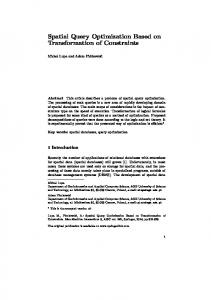
of these rules are identical as are the corresponding partitions. Then using Algorithm 5.3, we can see that if a(X2 X3 X1 X3 ) ! d(X2X3 X1 X3 ) holds, where d is the context de ned by d(X2 X3 X1 X3 ) :- b(X2 X3 X1 ); c(X3 X3 ), then r1 is contained in r2. 2 Example 7 Consider the pair of rules r1: p(X1 X2 X3 X4 ) :a1 (X1 X4 U), a2 (X2 X3 V ), a3(UV W), a4 (X3 X2 ), a5 (X4 X1 ), p(X1 X2 X3 X4 ) (see Fig. 5.2) and r2 : p(X1 X2 X3 X4 ) :- b1 (X1 X3 ), b2(X2 X4 ); b3 (X3 X2 ), b4 (X4 X1 ), p(X1 X2 X3 X4 ). It can be seen that (i) the sets of active variables of the rules are the same and (ii) the active variable partition induced by r2 is a re nement of that of r1. Following the algorithm, the CDs to be tested are: a(X1 X4 U); a2(X2 X3 V ); a3(UV W) ! b1 (X1 X3 ) a1 (X1 X4 U); a2(X2 X3 V ); a3(UV W) ! b2(X2 X4 ) a4 (X3 X2 ) ! b3(X3 X2 ) a5 (X4 X1 ) ! b4(X4 X1 ). If these CDs are implied by given constraints, then the algorithm will conclude that r1 is contained in r2 . 2 0
0
0
0
0
0
0
0
0
0
0
0
0
0
0
0
0
0
0
0
0
0
0
0
0
0
0
0
0
0
0
0
0
0
0
p * X’ 1 a1
* X4 *U
a
2
* X’ 2
* X’ 3
* X’ 4
* X3
* X2
* X1 a4
*V
*W
a5
a3
Fig. 5.2
6 Conclusions and Future Research We motivated the problem of carrying out semantic query optimization of programs in deductive databases that is independent of the particular query being processed or any query processing strategy used. In this context, we illustrated the use of INDs and CDs and developed an inference mechanism capable of inferring CDs from given INDs as well inferring new CDs from given ones. For a class of linear recursive programs we developed su�cient conditions for detecting redundant atoms in the rules of a program and for detecting redundant rules in a program. We also developed polynomial time algorithms to perform semantic optimization based on our characterizations. Our algorithms can be combined to give a powerful optimization tool for detecting and eliminating the two fundamental sources of redundancy in programs, in the presence of given constraints. Extending our su�cient conditions to necessary and su�cient conditions (for the properties being tested) while preserving the polynomial time complexity of the resulting algorithms is an interesting open problem. It would also be interesting to extend these results to larger classes of programs and integrity constraints. Finally, consider an existential predicate in a rule such that of the several CDs
generated by the redundancy testing algorithm, only some are implied by given constraints. In this case, the existential subgoal may be needed a bounded number of times w.r.t. the recursive predicate. Characterizing the conditions under which this happens, and the exact bound, as well developing a strategy for transforming the original program into an equivalent one where the latter program never uses the particular existential predicate more than the bound number of times is an interesting open problem.
References
[BR 86] F. Bancilhon and R. Ramakrishnan, \An amateur's introduction to recursive query processing strategies," ACM-SIGMOD Conf., 1986, pp. 16-52. [CGT 89] S. Ceri, G. Gottlob, and L. Tanca, \What You Always Wanted to Know About Datalog (And Never Dared to Ask)," IEEE Trans. Knowledge and Data Eng., (March 1989), 146-166. [CFP 84] M. Casanova, R. Fagin, and C. Papadimitriou, \Inclusion dependencies and their interaction with functional dependencies," JCSS 28,1 (1984), 9-59. [CGM 88] U.S. Chakravarthy, J. Grant, and J. Minker, \Foundations of semantic query optimization for deductive databases," in Foundations of Deductive Databases and Logic Programming, (ed. J. Minker), Morgan Kau�man, 1988, pp. 243-274. [CGM 90] U.S. Chakravarthy, J. Grant, and J. Minker, \Logic Based Approach to Semantic Query Optimization," ACM TODS, (June 1990), 162-207. [DDLM 87] A. D'Atri, P. Di Felice, V.S. Lakshmanan, and M. Moscarini, \Global context dependencies and their properties," Proc. 1st Symp. Math. Foundations of Database Systems, Dresden, GDR, Jan 1987. [GM 91] R. Godin and R. Missaoui, \Semantic query optimization using inter-relational functional dependencies," Proc. Hawaii Int. Conf. on System Sciences (HICSS-24), Jan 8-11, 1991, vol. III, pp. 368-375. [L 91] V.S. Lakshmanan, \Semantic Query Optimization Using Inclusion, Context, and Global Context Dependencies in Deductive Databases," Tech. Rep., Dept. of Comp. Science, Concordia University, Jan. 1991. [LH 91] V.S. Lakshmanan and H. Hernandez, \Structural Query Optimization: A Uniform Framework for Semantic Query Optmization in Deductive Databases," Proc. ACM SIGACT-SIGMOD Symp. Principles of Database Systems, Denver, May 29-31, 1991, pp. 102-114. [LH 88] S. Lee and J. Han, \Semantic query optimization in recursive databases," Proc. IEEE Int. Conf. Data Eng., 1988, pp. 444-451. [LHQ 91] S.-G. Lee, L.J. Henschen, and G.Z. Qadah, \Semantic Query Reformulation in Deductive Databases," Proc. IEEE Int. Conf. Data Eng., April 8-12, 1991, Kobe, Japan, pp. 232-239. [S 87] Y. Sagiv, \Optimizing datalog programs," 6th PODS, 1987, pp. 349-362. [Sh 86] O. Shmueli, \Decidability and Expressiveness Aspects of Logic Queries," Proc. ACM SIGACT-SIGMOD Symp. Principles of Database Systems, 1986, 237-249. [T 91] S. Tsur, \Deductive Databases in Action," PODS 1991 Invited Talk, Proc. ACM SIGACT-SIGMOD Symp. Principles of Database Systems, Denver, May 29-31, 1991,
pp. 142-153. [U 88-89] J.D. Ullman, Principles of Database and Knowledge-Base Systems, vol I & II, Comp. Sci. Press, MD., 1988-89. [V 88] M.Y. Vardi, \Fundamentals of dependency theory," in Trends in Theor. Comp. Science, (ed. I. Borger), Comp. Sci. Press, MD., 1988.