Temple H. Fay, Stephan V. Joubert, and Andrew Mkolesia. Department of Mathematical .... (4) shows an innocuous appearing differential equation, due to John.
AMERICAN JOURNAL OF UNDERGRADUATE RESEARCH
VOL. 3, NO.4 (2005)
On Solving Systems of ODEs Numerically Temple H. Fay, Stephan V. Joubert, and Andrew Mkolesia Department of Mathematical Technology Tshwane University of Technology Private Bag x680 Pretoria 0001 SOUTH AFRICA Received: December 2, 2004
Accepted: January 12, 2005
ABSTRACT Many beginning courses on ordinary differential equations have a computer laboratory component in which the students are asked to solve initial value problems numerically. But little attention in texts is given to the question of how accurate such solutions are. In this article we offer a simple procedure that not only can provide a measure of accuracy, but also often produces superior numerical results. I.
INTRODUCTION
equations can give rise to completely erroneous numerical solutions which appear quite plausible when plotted (for an example, see [5]). Thus we feel it is important for a student, or other solver, to have a method of testing the accuracy of a numerically generated solution. One need not have a strong background in numerical analysis to understand that things can go wrong and we give a simple strategy for solving systems such as
Computer algebra systems such as Mathematica [1], Maple [2], MATLAB [3], and Derive [4], have made possible a revolution in the way beginning differential equations courses are being taught. The emphasis used to be on solution techniques for various classes of equations which made the courses primarily a potpourri of “recipes”. Today the emphasis is more upon systems, nonlinear equations, and computer explorations. Indeed, many courses now have a computer laboratory component where students are asked to solve nonlinear equations and systems. Many beginning texts discuss uniform step size numerical techniques such as Euler’s method, the improved Euler’s method, and many mention Runge-Kutta order 4 (without a derivation). But today’s computer algebra systems generally employ a suite of much more advanced algorithms than these, for example, Mathematica version 4.2 uses an Adams method of order 12 [1] to solve non-stiff systems. But advanced as these algorithms are, they are by no means infallible and even simple-appearing second order
•
x = f (x, y , t )
(1)
•
y = g (x, y , t ) Here t is the independent variable, which we refer to as “time”, and the dots refer to differentiation with respect to t. The strategy we outline will allow us to test the accuracy of numerical results, and indeed this strategy often produces a superior numerical result from the algorithm. II.
WORKING PRECISION
Setting the working precision is an attempt to control the local round-off or
1
AMERICAN JOURNAL OF UNDERGRADUATE RESEARCH
subject to the initial conditions x (0 ) = a
truncation error. When solving an ODE over a long time interval, the local error accumulates and the algorithm may eventually produce a false solution rather than the true numerical solution. Generally speaking, a PC’s default working precision is 16; this means that at each step of a calculation 16 digits are used and the user can generally expect the result to be accurate to 6 digits. Often such a low precision is insufficient to obtain accurate numerical solutions to an ODE. To obtain more accurate results, one has to resort to requesting higher precision; Mathematica permits the user to set the precision of the numbers used in calculation using an option named Working Precision (see [1]). If the working precision is set to N, then the result is expected to be accurate to N - 10 digits. But this is misleading because this accuracy is only for a single calculation, and accumulated error means that as an algorithm executes more steps, the inputs to the accurate computation are increasingly inaccurate. Of course there is a trade-off: the higher the working precision, the longer the calculations are, the more memory is required. Indeed with a large working precision, the algorithm may force the application to freeze or shut down the solver altogether. The authors in practice seldom use a working precision higher than 26. III.
•
and x (0 ) = b . The traditional approach is to numerically solve the 2×2 system •
x=y y = −f (x, y ) + g (t ) with
•
x (0 ) = a,
y (0 ) = b
In order to substitute back into the equation we need the second derivative of x, but this technique does not compute it. The following easy strategy produces the second derivative: differentiate equation (2) and solve the 3×3 system •
x=y •
y =z •
z=−
(3) • d {f (x, y )} + g (t ) dt
x (0 ) = a,
y (0 ) = b ,
z(0 ) = −f (a, b ) + g (0 ).
By doing so, we numerically compute the ••
second derivative of x, that is z = x . This means that we can compute the “residual” z + f(x,y) – g(t) and graphically observe the accuracy of our numerical solution. Some more details on this may be found in [6]. For a system such as equation (1), we introduce the two auxiliary variables
In this section we discuss our strategy for solving an initial value problem. We focus on second order ordinary differential equations, as these are the most often encountered types in beginning courses. But there is really no restriction on the order of the equation. The idea is that the only way we know to gauge the accuracy of a solution is to substitute back into the equation and observe if the equation is “satisfied”. Suppose we wish to solve a typical second order differential equation ••
•
y = x and
introduce the auxiliary variable
THE STRATEGY AND RESIDUAL
x + f x, x = g (t )
VOL. 3, NO.4 (2005)
•
u=x •
v=y and rather than solve the 2×2 system (1), we solve the 4×4 system •
x =u
(2)
•
u=
2
d dt
f (x, y ) =
∂ ∂x
f (x, y )u +
∂ ∂y
f (x, y )v
AMERICAN JOURNAL OF UNDERGRADUATE RESEARCH
•
y=
∂ ∂ d g ( x, y ) = g (x, y )u + g (x, y )v ∂x dt ∂y
VOL. 3, NO.4 (2005)
student investigation because just about everything that can go wrong does.
x (0 ) = a, y (0 ) = b, u (0 ) = f (a, b ),
•
(4)
Turning this equation into a 2×2 system,
v (0 ) = g (a, b )
•
x=y
Solving this system produces not just x and •
y as when solving (1), but also
(5)
•
y = y2 − x
•
x and y ,
and thus we can check the accuracy of the solution by examining the two residuals
it is easy to see that the origin in the phase plane is the only critical value and it is a center. There is a parabolic separatrix which divides the phase plane into two regions, one for closed bounded trajectories, the other for unbounded trajectories. But this is not at all obvious. It turns out that for each initial condition of the form (x(0),y(0)) = (x0, 0), the trajectory in the phase plane is given by the equation
•
x − f (x, y ) and •
y − g (x, y ). We conclude with a pair of typical examples to illustrate this. IV.
2
x − x + x = 0
••
(2 x
A SECOND-ORDER EQUATION
Equation (4) shows an innocuous appearing differential equation, due to John Polking of Rice University—discussed briefly in [7] and in some detail in [8]—which is a numerical nightmare, and hence useful for
+ 1) e 2 ( x − x ) − 2x − 1 + 2y 2 = 0. 0
0
(5)
A phase portrait is shown in Figure 1. The initial conditions x(0) = -1/2, y(0) = 0 determine the parabolic separatrix x = y2 – 1/2. Solving the system (5) for these initial
Figure 1. A phase portrait of trajectories described by equation (4) for equations (5).
3
AMERICAN JOURNAL OF UNDERGRADUATE RESEARCH
VOL. 3, NO.4 (2005)
with x(0) = 6.7 and y(0) = 0.5. This model has a center in the population quadrant at (12, 0.5). A parametric plot of the solutions, x(t) versus y(t), is shown in Figure 4. Solving this system as it stands does not give an immediate way to test the accuracy of the solution, however by differentiating and solving the system
values, at machine default of precision 16, for 0 ≤ t ≤ 100, we obtain the trajectory shown in Figure 2 (a). Since we know the trajectory should be a parabola, this trajectory is clearly incorrect. Even increasing the working precision to 20 fails to produce the correct trajectory; it just takes longer to go off the mark. This is shown in Figure 2 (b). Solving the equivalent 3×3 system (3),
•
x =u
x=y y =z •
z = 2y
•
u = 0.405 u − 0.81(u y + x v )
(7)
•
•
v = − 1.5v + 0.125 (u y + x v )
z−y
with x(0) = 6.7, y(0) = 0.5, u(0) = 0, and v(0) = -0.331, we do indeed have a way to estimate the solution accuracy. Here we have introduced the auxiliary variables u =
with x(0) = -1/2,0 y(0) = 0, and z(0) = 1/2, at default precision 16, produces the correct trajectory shown in Figure 3. The residual zy2+x is bounded in absolute value by 2 × 10¹⁶ and indeed a plot of z shows it to be constant of value 1/2 as should be expected. Is this system just an accident? We invite the reader to solve the same systems using initial conditions
•
values u(0) = (0.405)(6.7) – (0.81)(5.7)(0.5) = 0 and v(0) = (-1.5)().5) + (0.125)(6.7)(0.5) = -0.331. In this way we numerically •
compute
x (0 ), x (0 ) = (6, 0 )
resid x (t ) = u − 0.405 x + 0.81x y
x (0 ), x (0 ) = (8, 0 ) •
resid y (t ) = v + 1.5 y − 0.125 x y
Plots of these residuals are shown in Figure 5 and suggest that, at least for 0 ≤ t ≤ 10, we have solutions x(t) accurate to 4 decimal places and y(t) accurate to 5 decimal places. We note that the solutions are periodic with period less than 10 so that these numerical solutions suffice if four decimal place accuracy suffices. To improve the accuracy, we would need to increase the working precision from a machine default of 16 to 20 or higher.
as representative. The 3×3 system out performs the 2×2 system in every case we have examined. A PREDATOR-PREY MODEL
Predator-prey models, competing species models, and other quadratic system models are now common fare in beginning courses. A model that we like to use in our courses is that for lions and wildebeest in Kruger National Park in South Africa. We let x(t) denote the population of wildebeest and y(t) denote the population of lions, measured in thousands. A predator-prey model has been developed [9] using data from park records to estimate coefficients •
•
x and y and are able to define the
pair of residuals
and
x = 0.405 x − 0.81x y
•
x and y = y and corresponding initial
•
V.
(9)
•
y =v
•
ACKNOWLEDGEMENTS The authors wish to thank the National Research Foundation of South Africa (NRF reference number 10334 GUN number 2054468) and the Tshwane University of Technology for supporting this work.
(8)
•
y = − 1.5 y + 0.125 x y
4
AMERICAN JOURNAL OF UNDERGRADUATE RESEARCH
VOL. 3, NO.4 (2005)
Figure 2. The 2×2 system of equation (5) with (a) working precision 16 [upper graph], and (b) working precision 20 [lower graph].
Figure 3. The 3×3 system, equation (7), at default precision 16, produces the correct trajectory.
5
AMERICAN JOURNAL OF UNDERGRADUATE RESEARCH
VOL. 3, NO.4 (2005)
Figure 4. A parametric plot of the solutions, x(t) versus y(t), of the predator-prey system described by system of equations (8), with working precision 16.
0.000015 0.000010 0.5×10⁻⁶ t
0 -0.5×10⁻⁶ 0
2
4
6
8
1×10⁻⁶ 0.5×10⁻⁶ 0
t
-0.5×10⁻⁶ -1×10⁻⁶ -1.5×10⁻⁶ -2×10⁻⁶ 0
2
4
6
8
Figure 5. The residuals residx(t) [top] and residy(t) [bottom], for 0 ≤ t ≤ 10, with working precision 16.
6
AMERICAN JOURNAL OF UNDERGRADUATE RESEARCH
REFERENCES
VOL. 3, NO.4 (2005)
ODEs,” New Zealand Journal of Mathematics 32 (Supplementary issue, November), pp. 67-75 (2003). 7. Knapp, R, and S. Wagon, “Check you answers…But how?” Mathematica In Action for Issue 7-4 of Mathematica in Education and Research (2001). 8. Schwalbe, D., and S. Wagon, VisualDSolve: Visualizing Differential Equations with Mathematics (Springer/TELOS, New York, 1997). 9. Fay, T.H. and J.C. Greeff, “Lions and Wildebeest: A Predator-Prey Model,” Mathematics and Computer Education 33, pp. 106-119 (1999).
1. Wolfram, S., The Mathematica Book, 3rd edn. (Wolfram Media/Cambridge University Press, New York, 1996). 2. Maple, version 9.5 (2004), www.maplesoft.com. 3. MATLAB, version 7 (2004), www.mathworks.com. 4. Dervie, version 6 (2004), www.deriveeurope.com. 5. Fay, T.H. and S.V. Joubert, “Square Waves from a Black Box,” Mathematics Magazine 73, pp. 393-396 (2000). 6. Fay, T.H. and S.V. Joubert, “Postanalysis of numerical solutions to
Tshwane University of Technology (TUT)
is the largest residential higher education institution in South Africa, with approximately 60 000 students. It is well positioned to meet the higher education needs of different communities in South Africa, with well-equipped campuses in Pretoria West (Pretoria Campus), Soshanguve, Ga-Rankuwa, Witbank, Nelspruit and Polokwane. Two faculties, namely the Faculties of Natural Sciences and Arts, have dedicated campuses in the Pretoria city center. As a higher education institution, TUT has a legal responsibility to conduct teaching and learning, and to undertake research and development and community service projects. TUT tries to do this in a unique way to strengthen its market position. TUT publicly commits itself to becoming the leading higher education institution in Southern Africa.
7
AMERICAN JOURNAL OF UNDERGRADUATE RESEARCH
8
VOL. 3, NO.4 (2005)