Aug 15, 1998 - we will introduce our generalized concatenation structure and give a formula ... Consider a linear (n, N) block code C with code rate Rc = N/n and minimum distance hm. ... for Concatenated Codes With Random Interleavers.
TMO Progress Report 42-134
August 15, 1998
On the Design of Concatenated Coding Systems With Interleavers D. Divsalar1 and R. J. McEliece2
In this article, we will study a class of concatenated coding communications systems that is built from convolutional codes and interleavers. These systems include as special cases both the classical turbo codes [1,2] and the serial concatenation of convolutional codes [4]. Our main results are a method for computing a conjectured interleaving gain exponent and for optimizing the effective free distance, d2 . We include proofs of theorems about d2 that were stated without proof in [6].
I. Introduction Our goal in this article is to introduce a class of generalized concatenated convolutional coding systems with interleavers that includes both parallel concatenated convolutional codes (turbo codes) [1,2] and serial concatenated convolutional codes [4] as special cases. We estimate the average (over all interleavers) performance of these codes using the classical union bound technique, which leads us to two important design parameters: the interleaving gain exponent, βM , and the effective free distance, hM . We shall see that these parameters are relatively easy to compute, and so they can serve the design engineer as preliminary figures of merit. Here is an outline of the article. In Section II, we will briefly review the union bound, as it applies to block codes, and see the importance of the input–output weight enumerator (IOWE). In Section III, we will introduce our generalized concatenation structure and give a formula for the average (over the ensemble of all interleavers) IOWE when the component codes are block codes. In Section IV, we will replace the block codes of Section III with truncated convolutional codes and study the parameters βM and hM mentioned above. In particular, we will show that, for both parallel and serial concatenation, hM is maximized if the d2 parameter of certain of the component codes is maximized. Then, in Section V, we will state and prove two uppper bounds on d2 that can be used to identify component codes with optimal or near-optimal values of d2 . Finally, in Section VI, we present tables of convolutional codes for which d2 is as large as possible.
II. Union Bounds on the Performance of Block Codes Consider a linear (n, N ) block code C with code rate Rc = N/n and minimum distance hm . The union bounds on the word-error probability, PW , and bit-error probability, Pb , of the code C over a memoryless binary-input channel, using maximum-likelihood decoding, have the well-known form 1 Communications 2 California
Systems and Research Section.
Institute of Technology and Communications Systems and Research Section.
1
n N X X
PW ≤
Aw,h z h
(1)
h=hm w=1
Pb ≤
n N X X w Aw,h z h N w=1
(2)
h=hm
where Aw,h denotes the number of codewords in C with input weight w and output weight h. The Aw,h ’s are called the input–output weight coefficients (IOWCs). The function z h represents an upper bound on the pairwise error probability for two codewords separated by Hamming (output) distance h. For additive white Gaussian noise (AWGN) channels, we have z = e−Rc Eb /N0 , where Eb /N0 is the signal-tonoise ratio per bit. For independent Rayleigh fading channels, assuming coherent detection, and perfect estimate of fading samples, we have z = [1 + Rc Eb /N0 ]−1 . All these results apply to convolutional codes as well, if we construct an equivalent block code by terminating the convolutional code. These results also apply to concatenated codes including parallel [1,2] and serial [4] concatenations and other types of code concatenations. C for Concatenated Codes With Random Interleavers III. Computation of Aw,h In this section, we consider a general class of concatenated coding systems of the type depicted in Fig. 1, with q encoders (circles) and q − 1 interleavers (boxes). The ith code Ci is an (ni , Ni ) linear block code, and the ith encoder is preceded by an interleaver (permuter) Pi of size Ni except for C1 , which is not preceded by an interleaver but rather is connected directly to the input. The overall structure must have no loops, i.e., it must be a graph-theoretic tree. P3 INPUT
w
w1
N
N1
C1
h1 n1 P4
P2
w2 N2
C2
h3
w3
C3
N3
OUTPUT
n3 h4
w4
C4
N4
OUTPUT
n4
h2 OUTPUT
n2
Fig. 1. An example of concatenated codes with tree structure sI = {1,2}, sO = {2,3,4}, and sO = {1}.
Define sq = {1, 2, · · · , q} and subsets of sq by sI = {i ∈ sq : Ci connected to input}, sO = {i ∈ sq : sO . The overall system depicted in Fig. 1 is then an encoder Ci connected to output}, and its complement P for an (n, N ) block code with n = i∈sO ni . (i)
If we know the IOWC’s Awi ,hi ’s for the constituent codes Ci , we can calculate the average IOWC’s Aw,h for the overall system (averaged over the ensemble of all possible interleavers), using the uniform interleaver technique [2]. (A uniform interleaver is defined as a probabilistic device that maps ¡ ¢a given ¡ ¢ input word of weight w into all distinct Nwi permutations of it with equal probability p = 1/ Nwi .) The result is
Aw,h =
X
X
hi :i∈sO Σhi =h
hi :i∈sO
2
(1)
Aw1 ,h1
(i) q Y Awi ,hi ¡Ni ¢ i=2
wi
(3)
In Eq. (3), we have wi = w if i ∈ sI , and wi = hj if Ci is preceded by Cj (see Fig. 2.). For example, for the (n2 + n3 + n4 , N ) encoder of Fig. 1, the formula of Eq. 3 becomes
Aw,h =
X
(2)
(3)
(4)
X
w2
w3
w4
h1 ,h2 ,h3 ,h4 (h2 +h3 +h4 =h)
Aw ,h Aw ,h Aw ,h (1) Aw1 ,h1 ¡N22 ¢2 ¡N33 ¢3 ¡N44 ¢4 =
h1 ,h2 ,h3 ,h4 (h2 +h3 +h4 =h)
(2)
(3)
(4)
w
h1
h1
(1) Aw,h Ah ,h Ah ,h Aw,h1 ¡N ¢2 ¡n11 ¢ 3 ¡n11 ¢ 4
¡ i¢ (i) (The formula of Eq. (3) is intuitively plausible if we note that the term Awi ,hi / N wi is the probability that a random input word to Ci of weight wi will produce an output word of weight hi .) Ci
hi
wj
Pj
ni
Cj
Nj
(n i , N i )
(n j , N j )
Fig. 2. Ci , an (ni , Ni ) encoder, is connected to Cj , an (nj , Nj ) encoder, by an interleaver of size Nj . We have the "boundary conditions" Nj = ni and wj = hi .
IV. Design of Concatenated Codes In this section, we will consider systems of the form depicted in Fig. 1, in which the individual encoders are terminated convolutional encoders, and study the behavior of the average IOWCs in Eq. 3 as the input block length N approaches infinity. To this end, we define, for each fixed w and h,3 β(w, h) = lim logN AC w,h N →∞
(4)
Two fundamental design parameters that we shall study here are βM = max max β(w, h)
(5)
hM = min{h : β(w, h) = βM for some w}
(6)
w
h
and
Extensive numerical simulations, and theoretical considerations that are not fully rigorous (see, e.g., [2] and [4]), lead us to make the following conjecture about the behavior of the union bounds, Expressions (1) UB and PbU B . and (2), for systems of the type shown in Fig. 1, which we denote by PW Conjecture 1. There exists a positive number z0 , which depends on the q component convolutional codes and the tree structure of the overall system, but not on N, such that, for any fixed z < z0 , as the block length N becomes large,4 3 Note
that the β’s in this article are exactly 1 more than the α’s in [3] and [4].
4 Because
of the inherent properties of the union bound, z0 will presumably be less than the “cutoff rate,” which for a binary code of rate r is zcutoff = 21−r − 1. 3
UB PW = O(N βM )
(7)
PbU B = O(N βM −1 )
(8)
Equation (7) says that if βM < 0, then, for a given z < z0 , the word-error probability of the concatenated code decreases to zero as the input block size is increased. Equation (8) says that, if the weaker condition βM < 1 is satisfied, the bit-error probability dereases to zero as the input block size is increased. When βM < 0, we say we have word-error probability interleaving gain, and when βM < 1, we say we have bit-error probability interleaving gain. Furthermore, by Eq. (6), the terms in the union bound of order N βM will be multiplied by z hM , so for a fixed value of βM , one expects systems with larger hM to perform better. In designing a system of the type depicted in Figure 1, our primary concern will be to minimize βM , and for a given value of βM , our secondary concern will be to maximize hM . We now shall discuss the calculation of β(w, h), βM , and hM for a concatenated system of the type depicted in Fig. 1, assuming that each of the encoders is a convolutional encoder. We use analytical tools introduced in [3] and [4]. Consider an (n, k, m) convolutional code C with rate R = k/n and memory m, and the corresponding sequence of (N/R, N − m) block codes C (N ) , for N = k, 2k, · · ·, obtained by truncating the convolutional code at depths L = 1, 2, · · ·. By definition, C (N ) consists of the output labels of the trellis paths from the all-zeros state back to the all-zeros state of length L = N/k. Let AC w,h,j be the input–output weight coefficients for those codepaths in the convolutional code C consisting of the concatenation of exactly j simple codepaths, with no gaps between them (see Fig. 3). We can “expand” each codepath of the type depicted in Fig. 3 into several codewords from C (N ) by inserting zero runs before each of the j simple codepaths, so that the overall path length is N/k. If the ith simple codepath starts in position li , then clearly 1 ≤ l1 < l2 < · · · < lj ≤
N k
(9)
¡ ¢ Since there are N/k set of indices satisfying Expression (9), we have the following bound on the IOWE j (N ) of the code C : (N )
Aw,h ≤
X µN/k ¶ j≥1
1
AC w,h,j
j
2
(10)
j
3 ERROR EVENT
w j hj w1
w3 h3
h1 w2 h2
j
S wi = w
INPUT WEIGHT
i =1
OUTPUT WEIGHT
j
S hi = h i =1
Fig. 3. A code sequence in the convolutional code C consisting of the concatenation of j C simple codepaths. The IOWC for such codepaths is denoted by Aw ,h , j .
4
Since in Eq. (4) w and h are fixed and N → ∞, we use the estimate µ ¶ N Nj ≈ j! j
(11)
Substituting this estimate into Expression (10), we obtain (N )
Aw,h ≈
X Nj AC j!k j w,h,j
(12)
j≥1
Using the estimate in Expression (12), and Expression (11) in Eq. (3) for each constituent code, we obtain
β(w, h) = max
( q X
ji (wi , hi ) −
i=1
q X i=2
X
wi :
) hi = h
(13)
i∈SO
where ji = ji (w, h) is defined by i ji (w, h) = max{j : AC w,h,j 6= 0}
Next we discuss the computation of the quantities ji (wi , hi ). For any convolutional code C, given a j-segment code sequence of the form depicted in Fig. 3, we have w1 + · · · + wj = w and h1 + · · · + hj = h. Thus, if wm denotes the minimum possible nonzero input weight that produces a finite-weight codeword, we have jwm ≤ w, so that j ≤ w/wm . Similarly, if hm denotes the minimum nonzero codeword weight, we have jhm ≤ h, so that j ≤ h/hm . Thus, we have ½¹ jC (w, h) ≤ min
º ¹ º¾ w h , wm hm
(14)
Note that if C is nonrecursive, we have wm = 1, whereas if C is recursive, wm = 2. Also, hm is the free distance of the code. Our object is to select the component codes so as to minimize βM , so that the bounds in Expressions (7) and (8) will be as small as possible. For example, consider the parallel concatenation of q codes, with q − 1 interleavers. If each of the component codes is recursive, then ji (wi , hi ) ≤ wi /2 and wi = w, for i = 1, · · · , q, and so by Expression (13), β(w, h) ≤ q
jwk 2
− (q − 1)w
Since this bound is a decreasing function of w ≥ 2, its maximum occurs for w = 2, so that βM ≤ −q + 2 (If any of the component codes is nonrecursive, a larger value of βM results). For a classical turbo code with q = 2, we have βM = 0, so by Eq. (7) there is no word-error probability interleaving gain. This 5
suggests that the word-error probability for classic turbo codes with a uniform interleaver will not improve with input block size, a fact that has been verified by numerical evaluations of the union bound. Thus, when all codes are recursive, to maximize the corresponding hM , we should maximize d2 , which is defined to be the minimum output weight for weight-2 input sequences for each constituent code. As another example, consider the serial concatenation of two convolutional codes. If the inner code is recursive, then we obtain from Eq. (13) β(w, h) = j o + j i − wi , where “o” denotes the outer code and “i” denotes the inner code. But by Expression (14), º ¹ oº h ho − ho + j +j −w ≤ dofree 2 ¹
o
i
i
where ho is the output weight of the outer encoder. This is a decreasing function of h0 ≥ dofree , so the minimum occurs at h0 = dofree , and so we have º ¹ o dfree + 1 +1 β(w, h) ≤ − 2 Therefore, for serial concatenated codes, if dof ≥ 3, βM ≤ −1, and there is interleaving gain for both bitand word-error probabilities. (If the inner code is nonrecursive, βM ≥ 0, and there is no interleaving gain.) Define di2 to be the minimum weight of codewords of the inner code generated by weight-2 input sequences. We obtain different values for hM for even and odd values of dof . Then using arguments similar to those leading to Expression (14), we find that for even dof , the output weight hM associated with the highest exponent of N is given by dof di2 2
(15)
(dof − 3)di2 + di3 2
(16)
hM = whereas for dof odd, the value of hM is given by
hM =
where di3 is the minimum weight of sequences of the inner code generated by a weight-3 input sequence. Thus, among inner codes with maximum d2 , we should choose those with maximum d3 . It follows from the arguments in this section that, in choosing the convolutional code fragments in Fig. 1, it is wise to choose those connected to the output to have feedback, and to have the largest possible value of d2 . In the next section (Section V), we will state and prove two theoretical results about the maximum possible value of d2 for an infinite impulse response (IIR) convolutional code fragment with given values of n, k, and m. Then, in Section VI, we will present some tables of IIR code fragments for which d2 has been maximized, and, for a given maximum value of d2 , d3 is maximized.
V. Two Upper Bounds on d2 In this section, we will prove two theorems about the quantity “d2 ” referred to in the previous section. (These theorems were stated without proof in [6].) We begin with some definitions. 6
An (r, k, m) binary convolutional code fragment5 is defined [8] as the set of all output sequences of r-vectors (x0 , x1 , · · ·) that can be produced by a fixed (r, k, m) convolutional encoder. An (r, k, m) convolutional encoder, in turn, is a linear sequential finite-state machine defined by four matrices, A, B, C, and D, with dimensions A:m×m B :k×m C :m×r D :k×r When the (A, B, C, D) encoder is presented with a sequence of k-dimensional input vectors u0 , u1 , · · ·, it moves through a sequence of m-dimensional state vectors in response and produces a sequence of r-dimensional output vectors. The sj ’s and the xj ’s are defined by the state–space equations sj+1 = sj A + uj B xj = sj C + uj D
(17)
for j = 0, 1, · · ·. (The initial state s0 is defined to be 0.) An output sequence x = (x0 , x1 , · · ·) sometimes is called a codeword. If the input sequence (uj ) and the state sequence (sj ) both become zero for all sufficiently large values of j, i.e, if uj = 0 and sj = 0 for all j ≥ L, then because of the linearity of the state–space equations, Eq. (17), it follows that xj = 0 for all j ≥ L. In that case, the sequence x = (x0 , x1 , · · · , xL−1 ) is called a finite codeword. Definition 1. If x is a binary vector or a finite sequence of binary vectors, the symbol |x| denotes the Hamming weight of x, i.e., the number of nonzero components of x. If u is the input to the encoder and x is the corresponding output, the codeword x is said to have input weight |u| and output weight |x|. Definition 2. For i ≥ 1, the input-weight-i minimum distance of the (A,B,C,D) code fragment is defined as di = min{|x| : |u| = i}
(18)
where, in Eq. (18), u is an input to the encoder and x is the corresponding output. Here are our two main results. Theorem 1. If C is a binary (r,k,m) convolutional code fragment, then µ» d2 ≤ min
¼ ¹ m−1 º¶ 2 2m r r, 2r + k k
(19)
use the term fragment to include the case of output dimension less than input dimension, i.e., r ≤ k, which commonly occurs in the construction of turbo-like codes.
5 We
7
Theorem 2. If C is a binary (r,1,m) convolutional code fragment with m ≥ 2, then d2 ≤ (2 + 2m−1 )r
(20)
Equality holds in Expression (20) if and only if the canonical generator matrix for the code fragment is of the form µ G(D) =
Pr (D) P1 (D) ,···, Q(D) Q(D)
where Q(D) is a primitive polynomial of degree m, and P1 (D), · · ·, Pm (D) are polynomials of degree m, each having constant term 1, none of which are equal to Q(D). The proof is organized as follows: In Section V.A, we define the state diagram and the zero-input state diagram for a given (A, B, C, D) encoder. Then in Section V.B, we give a (state-diagram) characterization of input-weight-2 codewords. In Section V.C, we give the heart of the proof of Theorems 1 and 2, in the case where the matrix A is nonsingular. Then, in Section V.D, we handle the case of singular A. Then, in Sections V.E and V.F, we put the pieces together and complete the proofs of the two main theorems. (We have relegated the proofs of two technical algebraic results to the Appendix.) A. The State Diagram and the Zero-Input State Diagram The state diagram corresponding to the (A, B, C, D) encoder defined in Eq. (17) is a finite, directed, labeled graph with 2m vertices and 2m+k (doubly labeled) edges. The vertices are (labeled by) the 2m possible states. If s is a state, and if u is an arbitrary k-vector, then there is a directed edge from s to s0 = sA + uB labeled (u, x), where x = sC + uD. Symbolically, we write s −→ s0 u x
where s0 = sA + uB x = sC + uD The zero-input (ZI) subdiagram of the state diagram has the same set of vertices as does the full-state diagram, but includes only those edges produced by inputs of the form u = 0. Thus, the ZI state diagram has 2m vertices and 2m edges, symbolically written as s −→ s0 0
x
where s0 = sA x = sC 8
For example, there is a simple (2, 1, 2) convolutional code defined by the four matrices µ A=
0 0
1 0
B = (1 µ C=
0)
1 1
0 1
D = (1
(21)
1)
whose state diagram and zero-input state diagram are shown in Fig. 4. (See also [8], Example 2.5.) 0/00 0/11
0
0/00
0
1/11
0
0/11
0/10 0
0
0/10
1
1
0
0
1
1
0
1/00
0/01
1
1/01
1
0/01
1
1
1/10
Fig. 4. The state diagram and the zero-input state diagram for the code defined in Eq. (21).
Here is a simple lemma we will need later on. Lemma 1. The total output weight of the 2 m zero-input edges is at most 2 m−1 . Equality holds if and only if each of the r columns of C has at least one nonzero entry. Proof. The set of output labels on the zero-input edges is exactly the set of 2m vectors x of the form x = sC, where s is an arbitrary binary m-vector. The ith component of sC is s · ci , where ci is the ith column on C. But the mapping s → s × c achieves the values 0 and 1 equally often, except when c is identically 0. The result now follows. ❐ A viewpoint we shall find useful is that of a codepath in the state diagram. A codepath is defined to be a path of finite length in the state diagram that begins and ends in the zero state. A typical codepath can be represented as follows: u
u
u
uL−1
x0
x1
x2
xL−1
0 1 2 s1 −→ s2 −→ · · · sL−1 −→ sL = 0 s0 = 0 −→
(22)
Note that the codepaths of length L are in one-to-one correspondence with the codewords of length L, the codeword associated with the codepath of Eq. (22) being (x0 , · · · , xL−1 ). 9
B. Some General Results on d2 Theorem 3. For a convolutional code fragment, d1 < ∞ if and only if for some row bi of B, bi AL = 0 for some nonnegative integer L. Proof. A finite codepath of input weight 1 must be of the form e
0
0
x0
x1
xL−1
i bi −→ bi A · · · −→ bi AL = 0 0 −→
❐
where ei is a k-vector of weight 1, with the “1” in the ith position. The next theorem characterizes the codepaths of input weight 2.
Theorem 4. The codepaths of input weight 2 are in one-to-one correspondence with the equations of the form bi Ati = bj Atj
(23)
where bi and bj are rows of B and ti and tj are nonnegative integers. (In Eq. (23), we assume (i,ti ) 6= (j, tj ).) Proof. An input sequence of weight 2 that produces a finite codepath must be either of the form (ei , 0, · · · , 0, ej , 0, · · · , 0) or else of the form (ei + ej , 0, · · · , 0) In the first case, the corresponding state sequence is e
ej
0
0
i bi −→ bi A · · · −→ bi At−1 −→ bi At + bj 0 −→
0
· · · −→ (bi At + bj )As = 0 From this it follows that bi At+s = bj As , as required. In the second case, the state sequence is ei +ej
0
0
0 −→ bi + bj −→ · · · −→ (bi + bj )At = 0 which is equivalent to bi At = bj At .
❐ 10
Theorem 5. Suppose that bi and bj are rows of B and that Eq. (23) holds, for two pairs (i,ti ) 6= (j, tj ). Then d2 ≤ r × (max(ti , tj ) + 1)
Proof. From Theorem 4, we see that Eq. (23) implies the existence of an input-weight-2 codepath of length max(ti , tj ) + 1. Naturally, the output weight of such a codepath cannot exceed r × (max(ti , tj ) + 1). ❐ Corollary 1. For any (r,k,m) convolutional code fragment with d1 = ∞, »
¼ 2m d2 ≤ r k
Proof. If {b1 , · · · , bk } are the rows of B, consider the set of k(L + 1) states of the form bi Aj , for i = 1, · · · , k, and j = 0, · · · , L. Each of these states is in the row space of A, and nonzero by Theorem 3, but since A is m × m, this row space contains at most 2m − 1 nonzero elements. Thus, if k(L + 1) ≥ 2m , the pigeon-hole principle implies that two of these states must be equal, i.e., there is an equation of the form bi As = bj At , with max(s, t) ≤ L. Then by Theorem 5, d2 ≤ (L + 1)r. Taking L + 1 = d2m /ke, we obtain the stated result. ❐ C. Nonsingular A In this section, we will assume that the matrix A is nonsingular. Theorem 6. If the matrix A is nonsingular, ¹
2m−1 r d2 ≤ 2r + k
º (24)
Proof. Let the k rows of B be denoted by B = {b1 , · · · , bk }. If two rows of B are equal, e.g., bi = bj , then by Theorem 5, d2 ≤ r, and so Expression (24) certainly is satisfied. Thus, from now on, we assume the rows of B to be distinct. If bi is the ith row of B, we denote by ti the least nonnegative integer t such that bi At ∈ B. (Such an integer must exist; e.g., bi An = bi , where n is the period of A.) If bi Ati = bj , we write j = π(i). We now associate with bi the following input-weight-2 codepath, which we call path Pi : Pi :
e
eπ(i)
i s0 = 0 −→ bi −→ · · · −→ bi Ati −1 −→ (bi Ati + bπ(i) ) = 0
0
0
(25)
We first note that each zero-input edge in the code’s state diagram occurs at most once among the k paths P1 , · · · , Pk . To see that this is so, assume the contrary, i.e., the existence of an equation of the form bi As = bj At 11
(26)
where i 6= j, s ≤ ti − 2, t ≤ tj − 2, and s ≥ t. Then, since we are assuming that A is invertible, we can multiply both sides of Eq. (26) by A−t and obtain bi As−t = bj
(27)
which contradicts the fact that ti is the least integer such that bi Ati ∈ B. Since each zero-input edge occurs at most once as an edge in {P1 , · · · , Pk }, and since by Lemma 1 the total output weight of all the zero-input edges is at most 2m−1 r, it follows that at least one of the k codepaths Pi has a total output weight corresponding to its zero input edges of at most b2m−1 r/kc. Since there are only two edges in Pi with nonzero input, the total output weight of Pi is, therefore, at most 2r + b2m−1 r/kc. ❐ D. Singular A In this section, we will assume that the matrix A is singular, i.e., rank (A) ≤ m − 1. Theorem 7. If the matrix A is singular, µ d2 ≤
» 1+
2m−1 k
¼¶ r
Proof. If {b1 , · · · , bk } are the rows of B, consider the set of kL states of the form bi Aj , for i = 1, · · · , k, and j = 1, · · · , L. Each of these states is in the row space of A, but since A is singular, this row space contains at most 2m−1 − 1 nonzero elements. Thus, if kL ≥ 2m−1 , the pigeon-hole principle implies that two of these states must be equal, i.e., there is an equation of the form bi As = bj At , with max(s, t) ≤ L. ❐ Then, by Theorem 5, d2 ≤ (1 + L)r. Taking L = d2m−1 /ke, we obtain the desired result. Lemma 2. If y is a real number, and if r is a positive integer, then dyer ≤ r + byrc
(28)
Proof. Write y = n + θ, where n is an integer and 0 < θ ≤ 1. Then dye = n + 1, byrc = nr + bθrc, and the inequality (28) becomes r − bθrc ≤ r ❐
which plainly is true. Corollary 2. If the matrix A is singular, ¹
2m−1 r d2 ≤ 2r + k
º
Proof. This follows from Theorem 7 and Lemma 2, where we set y = 2m−1 /k: 12
µ d2 ≤
» 1+
2m−1 k ¹
≤r+r+
¼¶ r
2m−1 r k
¹
2m−1 r = 2r + k
by Theorem 7
º by Lemma 2
º
❐ E. Proof of Theorem 1 Here we need only recapitulate. Corollary 1 tells us that » d2 ≤
¼ 2m r k
(29)
for any (r, k, m) convolutional code fragment. Theorem 6 tells us that ¹
2m−1 r d2 ≤ 2r + k
º (30)
holds when A is nonsingular, and Corollary 2 tells us that the same bound holds when A is singular. Thus, both Expressions (29) and (30) hold for any (r, k, m) convolutional code fragment. This proves Theorem 1. ❐ F. Proof of Theorem 2 We first note that the bound of Expression (20) is simply the second alternative in the bound of Expression (19) when k = 1, so that if equality holds in Expression (20), we must have »
¼ ¹ m−1 º 2 r 2m r ≥ 2r + k k
for k = 1, which simplifies to 2m−1 ≥ 2, i.e., m ≥ 2.6 Furthermore, if we apply the bound of Theorem 7 in the case of k = 1, we obtain d2 ≤ (1 + 2m−1 )r, which means that if d2 = (2 + 2m−1 )r, the feedback matrix A must be nonsingular. In summary, a necessary condition for an (r, 1, m) code fragment to have d2 = (2 + 2m−1 )r is that m ≥ 2 and that A be nonsingular. In the remainder of this section, we will assume that these two conditions are satisfied. Theorem 4 identifies the codepaths of input weight 2 in terms of equations of the form bi Ati = bj Atj
(31)
k = 1 and m = 1, the bound of Expression (20) can be improved to d2 ≤ r, with equality if and only if G(D) = (P1 (D)/(D + 1), · · · , Pr (D)/(D + 1)), where each Pi (D) equals either 1 or D. We omit the simple proof of this fact.
6 If
13
where bi and bj are rows of B. In the case of k = 1, however, B has only one row, which we shall denote by b. Furthermore, A is nonsingular, so that Eq. (31) can be simplified to bAt = b
(32)
If t is the least positive integer such that Eq. (32) holds, then the corresponding codepath is 1
0
0
0
d
bC
bAC
bAt−2 C
s0 = 0 −→ b −→ bA −→ · · · −→ bAt−1
1
−→
bAt−1 C+d
0
(33)
The output weight of this codepath is d2 = |d| + |bAt−1 C + d| + |bC| + |bAC| + · · · + |bAt−2 C| Since both d and bAt−1 C + d are r-vectors, we have |d| + |bAt−1 C + d| ≤ 2r Furthermore, since bC, bAC, · · · , bAt−2 C are output symbols on zero-input edges, it follows from Lemma 1 that |bC| + |bAC| + · · · + |bAt−2 C| ≤ 2m−1 r It therefore follows that d2 = 2r + 2m−1 r if and only if d = (1, 1, · · · , 1)
(34)
bAt−1 C = (0, 0, · · · , 0)
(35)
|bC| + |bAC| + · · · + |bAt−2 C| + |bAt−1 C| = 2m−1 r
(36)
and
The sum on the left side of Eq. (36) can be written as r X t−1 X
|bAi cj |
j=1 i=0
where cj is the jth column of C. Now according to Theorem A-1 in the Appendix, each of the sums Pt−1 i m−1 , which means that Eq. (36) holds if and only if i=0 |bA cj | is at most 2 t−1 X
|bAi cj | = 2m−1
i=0
14
for j = 1, · · · , r
(37)
But Theorem A-1 also says that Eq. (37) holds if and only if A is a primitive matrix and b and each of the cj ’s are nonzero. It therefore follows that necessary and sufficient conditions for d2 = (2 + 2m−1 )r are m ≥ 2 and A = a primitive m × m matrix b 6= 0 cj 6= 0
for j = 1, · · · , r
bA−1 cj = 0
for j = 1, · · · , r
d = (1, 1, · · · , 1)
(38)
What remains now is to translate the conditions of Eq. (38) into a statement about the code’s generator matrix. To do this, we use the fact that a generator matrix for a convolutional code fragment defined by the matrices (A, B, C, D) is given by ([8], Eq. (2.19)) ¤−1 £ × [c1 , · · · , cr ] + [1, · · · , 1] G(D) = b × D−1 Im − A
(39)
where b denotes the single row of B and cj is the jth column of C. Combining the fact that ¤−1 £ −1 −1 = D [Im − DA] with Theorem A-2, it follows from Eq. (39) that G(D) is of the D Im − A form µ G(D) =
Pr (D) P1 (D) ,···, Q(D) Q(D)
where Q(D) is a primitive polynomial of degree m (the characteristic polynomial of A), and Pj (D) = DPj0 (D)+Q(D), where Pj0 (D) is a polynomial of degree ≤ m−1. However, by Eq. (38) and Theorem A-2, the coefficient of Dm−1 in Pj0 (D) equals qm bA−1 cj = 0, so that Pj (D) has degree exactly m. Also, since the constant term of DPj0 (D) is 0, and the constant term of Q(D) is 1, it follows that the constant term of Pj (D) also is 1. Finally, since b 6= 0 and cj 6= 0, it follows from Theorem A-2 that Pj0 (D) 6= 0, so that ❐ Pj (D) 6= Q(D).
VI. Tables of “d2-Optimal” Convolutional Code Fragments In this section, we present Tables 1 through 7, giving the generator matrices (in octal notation) for a number of convolutional code fragments with the largest possible values of d2 .7 The entries in Table 1 for m ≤ 3 are identical to the corresponding entries in Table 2 of [3]. The entries in Tables 2, 4, and 7, with m ≤ 4, are taken from [5]. The entries in Table 5, and those in Tables 2, 4, and 7, with m = 5 or m = 6, are new. In every case, we have verified (theoretically in some cases and numerically in others) that the given value of d2 is maximal, even though that value may be strictly less than the bound of Theorem 1 7 In
the tables, we use the letter h to denote the entries of the generator matrices. This should not be confused with our previous use of h to denote the output weight of a codeword.
15
or Theorem 2, which is given by the db2 entry in the tables. (For (r, 1, 1) code fragments, the bound of Theorem 2 can be improved to d2 ≤ r, and we have given this as the value of db2 in Tables 1, 3, and 6.) In some cases, the maximum value of d2 can be obtained only by code fragments with repeated columns in the generator matrix. Unfortunately, experiment shows that using such code fragments as components of a turbo code yields poor results. Thus, when the optimal code fragment has repeated columns, we list it in italics, and immediately below, we give the best code fragment with the same parameters that does not have repeated columns. For two IIR code fragments with the same value of d2 , we would expect heuristically that the one with the highest value of d3 will give the best performance. Thus, in choosing the entries for the tables, when we found two or more code fragments with the largest possible value of d2 , we chose code fragments with the largest value of d3 . If the code fragment is used to build a systematic encoder, the free distance of the resulting code is dfree = mini (i + di ). In the tables, we denote the optimizing value of i by i∗ and the corresponding di by d∗ .8 For example, consider the m = 3 entry from Table 2. There we have h0 = 13 = D3 + D + 1, h1 = 15 = D3 + D2 + 1, and h2 = 17 = D3 + D2 + D + 1. Thus, the encoder fragment is
(D3 + D2 + 1) (D3 + D + 1)
G(D) = (D3 + D2 + D + 1)
(40)
(D3 + D + 1) and the corresponding (3, 2, 3) systematic encoder is G0 (D) =
1
0
0
1
(D3 + D2 + 1) (D3 + D + 1)
3 2 (D + D + D + 1)
(41)
(D3 + D + 1)
Table 2 says that the value of d2 for the encoder fragment is 3, so that the value of d2 for the (3, 2, 3) code with generator matrix given by Eq. (41) is d02 = 2 + d2 = 5. On the other hand, Table 2 says that d3 for the fragment is 1, so that dfree ≤ 3 + 1 = 4 for this code, and in fact dfree = 4 in this case. Table 1. The d2-optimal (1,1,m) code fragments. G = (h1 /h0 ) m
8 The
h0
h1
d2
db2
d3
(d∗ , i∗ )
1
3
2
1
1
∞
(1,2)
2
7
5
4
4
2
(2,3)
3
15
17
6
6
4
(2,4)
4
31
37
10
10
5
(2,4)
5
75
57
18
18
7
(4,4)
6
147
115
34
34
10
(4,5)
pair i∗ , d∗ may not be unique.
16
Table 2. The d2-optimal (1,2,m) code fragments.
³ G=
h1 /h0 h2 /h0
´
m
h0
h1
h2
d2
db2
d3
(d∗ , i∗ )
1
3
1
1
0
1
∞
(0,2)
2
7
3
5
2
2
0
(0,3)
3
13
15
17
3
4
1
(1,3)
4
23
35
27
6
6
2
(2,3)
5
45
43
61
10
10
3
(3,3)
Table 3. The d2-optimal (2,1,m) code fragments. G = ( h1 /h0 m
h0
h1
h2
h2 /h0 ) d2
db2
d3
(d∗ , i∗ )
1
3
2
1
2
2
∞
(2,2)
2
7
5
5
8
8
4
(4,3)
2
7
5
3
6
8
4
(4,3)
3
13
17
15
12
12
7
(7,3)
4
23
33
37
20
20
9
(6,4)
5
73
45
51
36
36
14
(6,5)
6
147
115
101
68
68
20
(6,5)
Table 4. The d2-optimal (1,3,m) code fragments.
à G=
h1 /h0 h2 /h0 h2 /h0
!
m
h0
h1
h2
h3
d2
db2
d3
(d∗ , i∗ )
2
7
5
3
1
1
2
0
(1,2), (0,3)
3
13
15
17
11
2
3
1
(2,2), (1,3), (0,4)
4
23
35
33
25
3
4
1
(1,3)
5
51
73
65
61
7
7
1
(1,3)
17
Table 5. The d2-optimal (2,2,m) code fragments.
³ G=
h1 /h0 h3 /h0
h2 /h0 h4 /h0
´
m
h0
h1
h2
h3
h4
d2
db2
d3
(d∗ , i∗ )
1
3
1
2
2
1
2
2
∞
(2,2)
2
7
3
3
5
5
4
4
0
(0,3)
2
7
1
5
5
3
3
4
1
(1,3)
3
15
3
11
11
13
7
8
3
(1,4)
4
31
35
23
23
21
12
12
3
(3,3)
Table 6. The d2-optimal (3,1,m) code fragments. G = ( h1 /h0 m
h0
h1
h2
h2 /h0
h3
h3 /h0 ) db2
d2
d3
(d∗ , i∗ )
1
3
2
1
1
3
3
∞
(3,2)
2
7
5
5
5
12
12
6
(6,3)
2
7
5
3
6
8
12
6
(6,3)
3
13
17
15
11
18
18
9
(9,3)
4
23
35
27
37
30
30
13
(10,4)
5
73
45
51
47
54
54
20
(10,5)
6
147
115
101
135
102
102
29
(11,5)
Table 7. The d2-optimal (1,4,m) code fragments.
h G=
1 /h0
h2 /h0 h3 /h0 h4 /h0
m
h0
h1
h2
h3
h4
d2
db2
d3
(d∗ , i∗ )
1
3
1
1
1
1
0
1
∞
(0,2)
2
7
5
5
5
5
0
1
2
(0,2)
2
7
1
2
3
5
0
1
0
(0,2)
3
13
15
17
11
7
2
2
0
(0,3)
4
23
35
33
37
31
3
4
1
(1,3)
5
51
47
61
63
75
5
6
1
(1,3)
18
VII. Conclusions In this article, we have introduced a class of concatenated coding systems that includes both classical “parallel” turbo codes and “serial” turbo codes. We have defined the important parameters βM (the interleaving exponent) and hM (the effective free distance) for these systems. Finally, we stated and proved two upper bounds on the “d2 parameter” for the component convolutional codes, which can be used to design systems with large hM .
References [1] C. Berrou, A. Glavieux, and P. Thitimajshima, “Near Shannon Limit ErrorCorrecting Coding: Turbo Codes,” Proc. 1993 IEEE International Conference on Communications, Geneva, Switzerland, pp. 1064–1070, May 1993. [2] S. Benedetto and G. Montorsi, “Unveiling Turbo Codes: Some Results on Parallel Concatenated Coding Schemes,” IEEE Trans. on Inf. Theory, vol. 42, pp. 409– 429, March 1996. [3] S. Benedetto and G. Montorsi, “Design of Parallel Concatenated Convolutional Codes,” IEEE Transactions on Communications, vol. 44, no. 5, pp. 591–600, May 1996. [4] S. Benedetto, D. Divsalar, G. Montorsi, and F. Pollara, “Serial Concatenation of Interleaved Codes: Performance Analysis, Design, and Iterative Decoding,” IEEE Trans. on Information Theory, vol. 44, no. 3, pp. 909–926, May 1998. [5] D. Divsalar and F. Pollara, “On the Design of Turbo Codes,” The Telecommunications and Data Acquisition Progress Report 42-123, July–September 1995, Jet Propulsion Laboratory, Pasadena, California, pp. 99–121, November 15, 1995. [6] D. Divsalar and R. J. McEliece, “On the Effective Free Distance of Turbo-Codes,” Electronics Letters, vol. 32, no. 5, pp. 445–446, February 29, 1996. [7] R. A. Horn and C. R. Johnson, Matrix Analysis, Cambridge: Cambridge University Press, 1988. [8] R. J. McEliece, “The Algebraic Theory of Convolutional Codes,” Chapter 12 in Handbook of Coding Theory, V. S. Pless and W. C. Huffman, eds., Amsterdam: Elsevier Science B.V., 1998. [9] E. Selmer, Linear Recurrence Relations Over Finite Fields, Bergen, Norway: University of Bergen Department of Mathematics, 1966.
19
Appendix Proofs of Theorems A-1 and A-2 In this Appendix, we shall give proofs of two results that we used in the proofs in Section V. Theorem A-1. If A is a nonsingular binary m × m matrix with period n, and if b and c are arbitrary nonzero m-vectors, and if t is an integer ≤ n, then |bc| + |bAc| + · · · + |bAt−1 c| ≤ 2m−1 with equality possible only if A is similar to the companion matrix of an mth degree primitive polynomial. Proof. Suppose that the minimal polynomial of A is Q(x), where Q(x) = xk − h1 xk−1 − · · · − hk where hk 6= 0 and k ≤ m. Then we have
Aj =
k X
hi Aj−i
for all j ≥ k
i=1
If we multiply this matrix equation on the left by b and on the right by c, and if we define xj = bAj c, we obtain
xj =
k X
hi xj−1
for all j ≥ k
i=1
Thus, x = (x0 , x1 , · · · , xn−1 ) is a nonzero codeword in the (n, k) cyclic code with parity-check polynomial equal to h(x). Then by a known result about cyclic codes ([9, pp. 81–83], |x| ≤ 2k−1 , with equality iff h(x) is primitive. Thus, since k ≤ m, we can have |x| = 2m−1 iff k = m and h(x) is a primitive polynomial of degree m. But since A is m × m, it follows that both the minimal and characteristic polynomials of A are equal to h(x), so that A is similar to the companion matrix of an mth-degree primitive polynomial. ❐ Theorem A-2. If A is a nonsingular nonderogatory9 m × m matrix with characteristic polynomial Q(D) = 1 − q1 D − · · · − qm Dm and if b and c are arbitrary m-vectors, then the rational function Fb (D) = b(Im − DA)−1 c is of the form 9A
nonderogatory matrix is one for which the characteristic and minimal polynomials are equal [7].
20
Pb,c (D) Q(D) where Pb,c (D) is a polynomial of degree ≤ m−1. The coefficient of 1 in Pb,c (D) is bc, and the coefficient of Dm−1 in Pb,c (D) is qm bA−1 c. Finally, if Q(D) is irreducible, then Pb,c (D) is the zero polynomial if and only if one or both of b and c are zero. Proof. We have (Im − DA)−1 = I + AD + A2 D2 + · · · so that Pb,c (D) =
X
(bAj c)Dj
j≥0
=
X
fj Dj
(say)
(A-1)
j≥0
Now since Q(D) is the characteristic polynomial for A, we have At = q1 At−1 + · · · + qm At−m ,
for t ≥ m
(A-2)
Combining Eqs. (A-1) and (A-2), we obtain ft = q1 ft−1 + · · · + qm ft−m ,
for t ≥ m
Hence, if we multiply Pb,c (D) by Q(D), we obtain a polynomial of degree ≤m − 1: Pb,c (D)Q(D) = f0 + (f1 − q1 f0 )D + · · · + (fm−1 − q1 fm−2 − · · · − qm−1 f0 )Dm−1 = g0 + g1 D + · · · + gm−1 Dm−1
(A-3)
If we recall that fj = bAj c, it follows from Eq. (A-3) that g0 = bc
(A-4)
g1 = b(A − q1 I)c .. . gm−1 = b(Am−1 − q1 Am−2 − · · · − qm−1 Im )c 21
(A-5)
Equation (A-4) shows that the coefficient of 1 in Pb,c (D), i.e., g0 , is bc. To prove the assertion about the coefficient of Dm−1 , i.e., gm−1 , observe that if we multiply Eq. (A-2) with t = m by A−1 , we obtain qm A−1 = Am−1 − q1 Am−2 − · · · qm−1 Im Substituting this expression into Eq. (A-5), we find that gm = qm bA−1 c, as asserted. Lastly we assume that Q(D) is irreducible and investigate the possibility that, for a fixed pair (b, c), the polynomial Pb,c (D) is identically zero. By Eq. (A-1), this is equivalent to bAj c = 0
for j = 0, 1, · · ·
(A-6)
But by a known result, if the minimal polynomial of A has degree m and is irreducible, and if c 6= 0, the vectors c, Ac, · · · , Am−1 c are linearly independent ([9, Chapter 7]). Thus, if Eq. (A-6) holds, it must be ❐ that b = 0. In summary, Pb,c (D) = 0 if and only if either b or c (or both) is zero.
22