parameters using measurements of the line active power response from small step reactance changes. The estimation methods are verified using simple grid ...
1
Estimation of Grid Parameters for the Control of Variable Series Reactance FACTS Devices Nicklas P. Johansson, Student Member, IEEE, Hans-Peter Nee, Senior Member, IEEE, Lennart Ängquist, Non-member
Abstract—For high performance control of Flexible AC Transmission System (FACTS) devices with controllable reactances, a representation of the surrounding grid is essential. Using such a model, an adaptive control strategy can be developed which optimizes the control in real time as the grid parameters change. This paper proposes such a generic grid model and derives the theory of how to estimate the main parameters using measurements of the line active power response from small step reactance changes. The estimation methods are verified using simple grid models in PSCAD simulations and more advanced grid models using SIMPOW simulations of a modified version of the CIGRE Nordic 32 grid. This work should be thought of as a foundation for developing control systems for variable series reactance FACTS devices. Index Terms- parameter estimation, power system stability, power transmission control, prediction methods, FACTS
I. INTRODUCTION
F
ACTS – Flexible AC Transmission System devices for power quality improvement and power flow control have attracted an increasing interest during the last decade. It is well known that power flow can be controlled and oscillations can be damped using controllable reactive elements inserted in series with the line in order to vary the effective reactance of the line. For example TCSC – Thyristor Controlled Series Compensation devices can be used as described in [2]. Most authors focus on the control of such devices for stability improvement (e.g. [3], [4], [5], [6] and [7]). The performance of any power flow control scheme depends on the surrounding grid. When the grid parameters change, the system response also changes. For optimal control then an adaptive approach must be used. For this purpose a grid model is required. In this paper it is proposed that the grid is represented by a simple analytical model having only few parameters, which can be estimated from the active power response to small step changes in the inserted series reactance. The aim of this paper is to investigate the relevance of the proposed model when it is applied to a larger power system. To this end, model parameters are estimated from simulations of the active power step response for a small reactance change on a line in a power grid. The model is then used to analytically predict the dynamic system step response when a large reactance is inserted in series with the specific transmission line. The results of the predictions are then compared with simulation results of the same power grid event. This analysis is done for three different power grid
simulation models with different complexity. The analysis is presently restricted to the active power flow dynamics and disregards voltage magnitude changes in the system. II. THEORY A. Proposed Grid Model A simple grid model is proposed in Fig 1. The grid is represented by two synchronous machines with inertia constants H1 and H2. The inner reactance of each machine is included in the Xi parameter, which also includes the reactance in the grid outside the loop where the controllable reactance device is placed. The controlled line reactance is X. The total grid including lines, generation and loads, connected in parallel with the controlled line, is represented by the reactance Xeq. The voltages on the synchronous machine terminals are assumed to be well controlled. The resistive components of the line and machine impedances have been neglected. When applied to real power systems, the model can be thought of as a representation of two different areas with lumped moments of inertia and their connecting power lines. Here the power balance yields that the total average active power transfer, Ptot, between areas should be constant assuming a constant power dispatch between the areas. This power transfer is calculated as the average active power transfer over one period of any power oscillation on the line. The power flow through the reactance controlled line is denoted by Pline.
Fig 1: Proposed grid model with main parameters
B. Changes in average power flow with reactance change The basic relationship for the transmitted power on a purely reactive line is
P=
U1 j U 2 j sin(θ1 j − θ 2 j )
(1)
X
see for example in [1]. Here U1j and U2j are the node voltages θ θ in either end of the line, 1j and 2j are the voltage phase angles at the line terminals and X is the effective reactance of the line. If (1) is used to express the transmitted power on the parallel lines in Fig 1 it yields
2
Ptot =
U U sin(θ − θ )( X eq + X ) 1j 2 j 1j 2j . X eq X
(2)
The power transmitted on the controlled line is then given by
Pline =
U1 j U 2 j sin(θ1 j − θ 2 j )
.
(3)
X
Combination of (2) and (3) yields
X eq P P = line0 X + X tot eq 0
(4)
where X0 is the initial value of X and Pline0 is the initial power transmitted through the reactance controlled line. Ptot, the average transmitted power between the areas, is constant for any change in the reactance X. Equation (4) also applies to the transmitted power after a step in reactance such that X=X0+ ∆X . Accordingly,
X eq
= P P . line X + X + ∆X tot eq 0
U1U 2 sin(θ1 − θ 2 ) ≈ X tot
U U cos θ stat ( ∆θ1 − ∆θ 2 ) Pe0 + 1 2 X tot
(8)
θ θ θ linearising around an equilibrium point stat= stat1- stat2 with θ θ ∆ 1 and ∆ 2 as the deviations from the equilibrium points of θ θ the different machine electrical angles stat1 and stat2. Pe0 is the transmitted power at the equilibrium point. U1 and U2 are the voltages at the two machines and these are assumed to be constant in the following derivation.
Fig 2: Simplified two machine system with variable reactance transmission line
(5)
The two unit system equations, linearised around the θ equilibrium voltage angle difference stat, can then from (7) be expressed as
(6)
2 ω0 d ∆θ1 = Pe max cos(θ stat )( ∆θ 2 − ∆θ1 ) 2 2 H1 dt 2 ω0 d ∆θ 2 = Pe max cos(θ stat )( ∆θ1 − ∆θ 2 ) 2 2H 2 dt
Dividing (5) with (4) and rearranging yields
X eq + X 0 Pline ( X ) = Pline0 X eq + X + ∆X 0
Pe =
where Pline is the power transmitted through the reactance controlled line after the step ∆X. This expression can be used to estimate Xeq from measurements of the transmitted average active power on the line before and after a given step in reactance from X0 to X.
(9)
with
Pe max =
U1U 2 . X tot
(10)
C. Changes in dynamic power flow with reactance change In order to get a description of the dynamic properties of the system, the step response of the active power transmitted on the controlled line, when it is subject to a step in line reactance, will be derived.
Here Pemax is the maximum transmittable power on the line. It is assumed that the mechanical power to each machine balances the its electrical output power before the reactance change and that is remains constant.
If damping is neglected, the equation governing the electrical angle of a synchronous machine is written as
To start with, we solve the system of equations (9) with an initial condition which is non-stationary before the concept of a reactance step is introduced.
2 ω0 d θe = ( Pm − Pe ) . 2 2H dt
(7)
θ Here H is the inertia constant of the machine, e is the electrical angle of the machine, Pm is the mechanical power which is assumed constant, Pe is the electrical active power and ω0 is the base electrical angular frequency of the grid.
For a system like the one depicted in Fig 2, Pe can be expressed as
To solve this system of differential equations, Laplace transforms are used. In the frequency domain the system is: ω0 Pe max 2 s ∆θ1 ( s ) − s ∆θ10 = cos(θ stat )( ∆θ 2 ( s ) − ∆θ1 ( s )) 2 H1 . (11) ω P e max 2 s ∆θ 2 ( s ) − s ∆θ 20 = 0 cos(θ stat )( ∆θ1 ( s ) − ∆θ 2 ( s )) 2H 2
θ θ θ Here the initial values of are chosen to ∆ 1= ∆ 10 and ∆ 2= θ θ θ ∆ 20 and d∆ 1(t)/dt= d∆ 2(t)/dt=0 at t=0. Solving this linear θ system of equations with A=Pemaxcos statω0 /2 yields
3
2 ∆θ 20 A H1 + ∆θ10 ( s + A H 2 ) ∆θ1 ( s ) = 2 s ( s + A H1 + A H 2 ) 2 ∆θ10 A H 2 + ∆θ 20 ( s + A H1 ) ∆θ 2 ( s ) = 2 s ( s + A H1 + A H 2 )
(12)
If (12) is transformed to the time domain (using tables) it is found that ∆θ1 (t ) =
( ∆θ10 − ∆θ 20 ) cos ω t + ∆θ 20 + ∆θ10 H1 H 2 1 + H1 H 2
(13)
( ∆θ 20 − ∆θ10 ) cos ω t + ∆θ10 + ∆θ 20 H 2 H1 ∆θ 2 ( t ) = 1 + H 2 H1 Fig 3: Voltage angle dynamics when a sudden change in line reactance is applied starting from a stable equilibrium point
where ω=
A(
1 H1
+
1 H2
) =
U1U 2 cos θ stat ω0 1 1 ( + ) 2 X tot H1 H 2
(14)
θ Let the deviation from the equilibrium point stat of the total θ θ θ voltage angle between machines be ∆ osc(t)= ∆ 1(t)-∆ 2(t). Subtraction of the expressions in (13) gives
∆ θ osc ( t ) = ( ∆ θ10 − ∆ θ 20 ) cos ω t .
(15)
This yields the total angle difference including the equilibrium point
θ (t ) = ( ∆θ10 − ∆θ 20 ) cos ω t + θ stat .
(16)
When the line reactance is abruptly changed due to the connection of a series reactance, the equilibrium angle θ θ θ difference stat is changed to stat+ ∆ stat. From a stable ∆θ ∆θ situation when 10=0 and 20=0, an oscillation is induced around the new equilibrium point and (16) yields
θ (t ) = −∆θ stat cos ω t + θ stat + ∆θ stat .
(17)
An example of an oscillation of the machine electrical angles θ θ 1 and 2 induced by a change in the equilibrium voltage angle between the machines is schematically depicted in Fig 3. The equilibrium points of the voltage angles before and after the θ disturbance are shown in the figure and they are denoted stat1 θ θ θ and stat2 before the disturbance and stat1’ and stat2’ after the disturbance.
Now, in order to derive the exact expressions for the power oscillation, consider the system in Fig 1. If X is abruptly changed to X’, the power transfer on all lines change abruptly. The expression for the active power time dependence is calculated using (17). The calculation is based on the assumption that the total average active power transfer between areas (Ptot) before and after the reactance step is the same. The new average power transfer after the reactance step through the controlled line is given by (6). To this new average value, an oscillation is added, induced by the change in reactance. Initially, the expression for the total power oscillation between areas following a change in line reactance is derived. Now consider Fig 2. The change in equilibrium value of the θ θ total angle between generators from stat to stat’ when the reactance changes from Xtot to Xtot’ is derived from (8) with Ptot constant. If (8) is applied to the circuit in Fig 2 before and after the reactance step, linearising both expressions around θ the angle difference 0 and setting the power expressions equal it is found that sin θ stat X tot sin θ 0 X tot
+
=
sin θ stat ′ X tot ′
≈
cos θ 0 (θ stat − θ 0 ) = X tot
(18)
cos θ 0 (θ stat ′ − θ 0 ) X tot ′ X tot ′ θ θ Setting 0= stat in this expression and rearranging gives sin θ 0
+
θ stat ′ − θ stat =
X tot ′ − 1 cos θ stat X tot sin θ stat
(19)
θ Since sin stat can be expressed as a function of Ptot, Xtot, U1 and U2 from (8), (19) reduces to
4
∆θ stat =
(
Ptot X tot ′ − X tot U1U 2 cos θ stat
)
(20)
θ θ θ with ∆ stat= stat’- stat. Combining this with (17) and (8), the cosine term is eliminated and the power oscillation Posc(t) between machines, excluding the average power transfer, becomes
Posc (t ) =
U1U 2 ′ X tot
Ptot X tot U U 1 2
Ptot X tot ′ cos ω ′t (21) − U1U 2
with
ω′ =
U1U 2 cos θ stat′ω0 1 1 ( + ). H1 H 2 2 X tot ′
(22)
By using (1) for the different branches and eliminating, it is evident that after the step X ′X eq Ptot = PX X ′ (23) X ′ + X eq holds with PX denoting the power through the controlled line. This applies also for the oscillative part of the power transmitted on the controlled line PXosc(t) such that
Posc (t )
X ′X eq X ′ + X eq
= PX osc (t ) X ′
(24)
We can then derive the oscillation of power through the reactance controlled line using (21) and (24),
X eq
Ptot
(
PXosc (t ) = X tot − X tot X ′ + X eq X ′ tot
′
) cos ω ′t .
(25)
It is known that for the system in Fig 1,
X tot = X i +
XX eq
(26) X + X eq and for Xtot’ the same applies with X changed to X’. From (23) applied to the situation before the step, it can be deduced that
be calculated from (6), an expression for the step response in active power at t=t0 given a change in line reactance can be derived.
PX (t ) = PXstat
t