On the exact learnability of graph parameters: The case of partition functions ∗ Nadia Labai
†
arXiv:1606.04056v1 [cs.LG] 13 Jun 2016
Department of Informatics, Vienna University of Technology, Vienna, Austria
[email protected] Johann A. Makowsky
‡
Department of Computer Science, Technion - Israel Institute of Technology, Haifa, Israel
[email protected]
Abstract We study the exact learnability of real valued graph parameters f which are known to be representable as partition functions which count the number of weighted homomorphisms into a graph H with vertex weights α and edge weights β. M. Freedman, L. Lov´ asz and A. Schrijver have given a characterization of these graph parameters in terms of the k-connection matrices C(f, k) of f . Our model of learnability is based on D. Angluin’s model of exact learning using membership and equivalence queries. Given such a graph parameter f , the learner can ask for the values of f for graphs of their choice, and they can formulate hypotheses in terms of the connection matrices C(f, k) of f . The teacher can accept the hypothesis as correct, or provide a counterexample consisting of a graph. Our main result shows that in this scenario, a very large class of partition functions, the rigid partition functions, can be learned in time polynomial in the size of H and the size of the largest counterexample in the Blum-Shub-Smale model of computation over the reals with unit cost.
1
Introduction
A graph parameter f : G → R is a function from all finite graphs G into a ring or field R, which is invariant under graph isomorphisms. In this paper we initiate the study of exact learnability of graph parameters with values in R, which is assumed to be either Z, Q or R. As this question seems new, we focus here on the special case of graph parameters given as partition functions, [10, 13]. We adapt the model of exact learning introduced by D. Angluin [1]. Our research extends the work of [3, 11], where exact learnability of languages (set of words or labeled trees) recognizable by multiplicity automata (aka weighted automata) was studied, to graph parameters with values in R.
1.1
Exact learning
In each step, the learner may make membership queries value(x) in which they ask for the value of the target f on specific input x. This is the analogue of the membership queries ∗ This
is the complete version of the MFCS 2016 paper. by the National Research Network RiSE (S114), and the LogiCS doctoral program (W1255) funded by the Austrian Science Fund (FWF). ‡ Partially supported by a grant of Technion Research Authority. This work was done [in part] while the author was visiting the Simons Institute for the Theory of Computing. † Supported
1
used in the original model of exact learning, [2]. The learner may also propose a hypothesis h by sending an equivalent(h) query to the teacher. If the hypothesis is correct, the teacher returns “YES” and if it is incorrect, the teacher returns a counterexample. A class of functions is exactly learnable if there is a learner that for each target function f , outputs a hypothesis h such that f (x) = h(x) for all x and does so in time polynomial in the size of a shortest representation of f and the size of a largest counterexample returned by the teacher.
1.2
Formulating a hypothesis
To make sense one has to specify the formalism (language) L in which a hypothesis has to be formulated. It will be obvious in the sequel, that the restriction imposed by the choice of L will determine whether f is learnable or not. Let us look at the seemingly simpler case of learning integer functions f : Z → Z or integer valued functions of words w ∈ Σ⋆ over an alphabet in Σ. (i) If f can be any function f : Z → Z or f : Σ⋆ → Z, there are uncountably many candidate functions as hypotheses, and no finitary formalism L is suitable to formulate a hypothesis. P i (ii) If f is known to be a polynomial p(X) = i ai X ∈ Z[X], we can formulate the m hypothesis as a vector a = (a1 , . . . , am ) in Z . Learning is successful if the learner finds the hypothesis h = a in the required time. Here Lagrange interpolation will be used to formulate the hypotheses. (iii) If f is known to satisfy some recurrence relation, the hypothesis will consist of the coefficients and the length of the recurrence relation, and exact learnability will depend on the class of recurrence relations one has in mind. (iv) If f : Σ⋆ → Z is a word function recognizable by a multiplicity automaton M A, the hypotheses are given by the weighted transition tables of M A, cf. [3]. Looking now at a graph parameter f : G → R what can we expect? Again we have to restrict our treatment to a class of parameters where each member can be described by a finite string in a formalism L. We illustrate the varying difficulty of the learning problem with the example of the chromatic polynomial χ(G; X ∈ N[X]) for a graph G. For X = k, the evaluation of χ(G; k) counts the number of proper colorings of G with at most k colors. It is well known that for fixed G, χ(G; k) is indeed a polynomial in k, [4, 7]. A graph parameter f is a chromatic invariant over R if (i) it is multiplicative, i.e., for the disjoint union G1 ⊔ G2 of G1 and G2 , it holds that f (G1 ⊔ G2 ) = f (G1 ) · f (G2 ), and (ii) there are α, β, γ ∈ R such that f (G) = α · f (G−e ) + β · f (G/e ) and f (K1 ) = γ. Kn denotes the complete graph on n vertices, and G−e and G/e are, respectively, the graphs obtained from deleting the edge e from G and contracting e in G. The parameter χ(G; k) is a chromatic invariant with α = 1, β = −1 and γ = k. Finally, χ(G; k) has an interpretation by counting homomorphisms: X χ(G; m) = 1, t:G→Km
This is a special case of the homomorphism counting function for a fixed graph H: X hom(G, H) = 1, t:G→H
where t is a homomorphism t : G → H. Now, let a graph parameter f : G → R be the target of a learning algorithm.
2
1 u 1
1
v X Figure 1: The weighted graph Hindep .
(i) If f is known to be an instance of χ(G; X), a hypothesis consists of a value X = a. But in this case we know that χ(K1 ; X) = X, so it suffices to ask for f (K1 ) = a. (ii) If f is known to be a chromatic invariant, the hypothesis consists of the triple (α, β, γ). In this case a hypothesis can be computed from the values of f (Pm ) for undirected paths Pm for sufficiently many values of m. (iii) If f is known to be an instance of hom(−, H), a hypothesis would consist of a target graph H.
1.3
Counting weighted homomorphisms aka partition functions
A weighted graph H(α, β) is a graph H = (V (H), E(H)) on n = |V (H)| vertices together with a vertex weight function α : V (H) → R, viewed as a vector of length n, and an edge weights function β : V (H)2 → R viewed as an n×n matrix, with β(u, v) = 0 if (u, v) 6∈ E(H). A partition function1 hom(−, H(α, β)) is the generalization of hom(−, H) to weighted graphs, whose value on a graph G is defined as follows: Y X Y β(t(u), t(v)) α(t(v)) hom(G, H(α, β)) = t:G→H v∈V (G)
(u,v)∈V (G)2
To illustrate the notion of a partition function, let Hindep be the graph with two vertices {u, v} and the edges {(u, v), (u, u)}, shown in Figure 1. Let α(u) = 1, α(v) = X and β(u, v) = 1, β(u, u) = 1. Then hom(−, Hindep (α, β)) is the independence polynomial, X indj (G)X j hom(G, Hindep (α, β)) = I(G; X) = j
where indj (G) is the number of independent sets of size j in the graph G. We say a partition function hom(−, H(α, β)) is rigid aka asymmetric 2 , if H has no proper automorphisms. Note that automorphisms in a weighted graph also respect vertex and edge weights. In our examples above, the evaluations of the independence polynomial are rigid partition functions, whereas the evaluations of the chromatic polynomial are not. It is known that almost all graphs are rigid: Theorem 1 ([9, 12]). Let G be a uniformly selected graph on n vertices. The probability that G is rigid tends to 1 as n → ∞. If the target f is known to be a (rigid) partition function hom(−, H(α, β)) then the hypothesis consists of a (rigid) weighted graph H(α, β). In Section 2 we give the characterization of rigid and non-rigid partition functions from [10, 14, 13] in terms of connection matrices. For technical reasons discussed in Section 5, in this paper we deal only with the learnability of rigid partition functions, and leave the general case to future work. 1 In the literature hom(−, H(α, β)) is also denoted by Z H(α,β) (G), e.g., in [18]. We follow the notation of [13]. 2 Some authors say G is asymmetric if G has no proper automorphisms, and G is rigid if G has no proper endomorphisms, [12]. Wikipedia uses rigid as we use it here.
3
1.4
Main result
Our main result can now be stated: Theorem 2. Let f be a graph parameter which is known to be a rigid partition function f (G) = hom(G, H(α, β)). Then f can be learned in time polynomial in the size of H and the size of the largest counterexample in the Blum-Shub-Smale model of computation over the reals with unit cost. Remark 3. If f takes values in Q rather than in R we can also work in the Turing model of computation with logarithmic cost for the elements in Q. To prove Theorem 2 we will use the characterization of rigid partition functions in terms of connection matrices, [13, Theorem 5.54], stated as Theorem 4 and Corollary 6 in Section 2. The difficulty of our result lies not in finding a learning algorithm by carefully manipulating the counterexamples to meet the complexity constraints, but in proving the algorithm correct. In order to do this we had to identify and extract the suitable algebraic properties underlying the proof of Theorem 4 and Corollary 6. The learning algorithm is given in pseudo-code as Algorithm 1. It maintains a matrix M used in the generation of the hypothesis h from value and equivalent query results. After an initial setup of M , in each iteration the algorithm generates a hypothesis h, queries the teacher for equivalence between h and the target and either terminates, or updates M accordingly and moves on to the next iteration. Algorithm 1 Learning algorithm for rigid partition functions 1: n = 1 2: while True do 3: augment M with(Bn ) 4: P = find basis(M ) 5: h = generate hypothesis(P ) 6: if equivalent(h) = YES then 7: return h 8: else 9: n=n+1 10: Bn = equivalent(h) ⊲ Bn receives a counterexample 11: end if 12: end while It uses three black-boxes; find basis which uses M to find a certain basis P of a graph algebra associated with the target function (see Section 2), generate hypothesis which uses this basis and value queries to construct a hypothesis h, and augment M which augments the matrix M after a counterexample is received, using value queries. We briefly overview the complexity of the algorithm to illustrate that rigid partition functions are indeed exactly learnable. Proofs of validity and detailed analysis of the complexity are given in later sections. For a target H(α, β) on q vertices, the procedure find basis solves O(q) systems of linear equations, and systems of linear matrix equations, all of dimension O(poly(q)). The procedure generate hypothesis performs O(q) graph operations of polynomial time complexity on graphs of size O(poly(q, |x|)), where |x| is the size of the largest counterexample, and O(q 2 ) value queries. The procedure augment M performs O(q) value queries. Thus, each iteration takes time O(poly(q, |x|)). Lemma 18 will show that there are O(q) iterations, so the total run time of the algorithm is polynomial in the size q of H(α, β) and the size |x| of the largest counterexample. Organization In Section 2 we give the necessary background on partition functions and the graph algebras induced by them. Section 3 presents the algorithm in detail and in Section 4 we prove its validity and analyze its time complexity. We discuss the results and future work in Section 5. Some of the more technical proofs appear in Appendix A.
4
2
Preliminaries
Let k ∈ N. A k-labeled graph G is a finite graph in which k vertices, or less, are labeled with labels from [k] = {1, . . . , k}. We denote the class of k-labeled graphs by Gk . The k-connection of two k-labeled graphs G1 , G2 ∈ Gk is given by taking the disjoint union of G1 and G2 and identifying vertices with the same label. This produces a k-labeled graph G = G1 G2 . Note that k-connections are commutative.
2.1
Quantum graphs
A formal linear combination of a finite number of k-labeled graphs Fi ∈ Gk with coefficients from R is called a k-labeled quantum graph. Qk denotes the set of k-labeled P P quantum graphs. Let x, y be k-labeled quantum graphs: x = ni=1 ai Fi , and y = ni=1 bi Fi . Note that some of the coefficients dimensional vector space, Pn with the Pn Pn Qk is an infinite Pnmay be zero. and α · x = i=1 (αai )Fi . operations: x + y = ( i=1 ai Fi ) + ( i=1 bi Fi ) = i=1 (ai + bi )Fi , P n k-connections extend to k-labeled quantum graphs by xy = i,j=1 (ai bj )(Fi Fj ). Any P graph parameter f extends to k-labeled quantum graphs linearly: f (x) = ni=1 ai f (Fi ).
2.2
Equivalence relations for quantum graphs
The k-connection matrix C(f, k) of a graph parameter f : G → R is a bi-infinite matrix over R whose rows and columns are labeled with k-labeled graphs, and its entry at the row labeled with G1 and the column labeled with G2 contains the value of f on G1 G2 : C(f, k)G1 ,G2 = f (G1 G2 ). Given a connection matrix C(f, k), we associate with a k-labeled graph G ∈ Gk the (infinite) k row vector RG appearing in the row labeled by G in C(f, k). If k is clear from context we writePRG . Similarly, we associatePan infinite row vector Rx with k-labeled quantum graphs n n x = i=1 ai Fi , defined as Rx = i=1 ai RFi where RFi is the row in C(f, k) labeled by the k-labeled graph Fi . We say C(f, k) has finite rank if there are finitely many k-labeled graphs BC(f,k) = {B1 , . . . , Bn } whose rows RC(f,k) = {RB1 , . . . , RBn } linearly span C(f, k). Meaning, for any k-labeled graph G, there exists a linear combination of the rows in RC(f,k) which equals the row vector RG . We say that C(f, k) has rank n and denote r(f, k) = n if any set of less than n graphs does not linearly span C(f, k). The main result we use is the characterization of partition functions in terms of connection matrices. We do not need its complete power, so we state the relevant part: Theorem 4 (Freedman, Lov´asz, Schrijver, [10]). Let f be a graph parameter that is equal to hom(−, H(α, β)) for some H(α, β) on q vertices. Then r(f, k) ≤ q k for all k ≥ 0. The exact rank r(f, k) was characterized in [14], but first we need some definitions. A weighted graph H(α, β) is said to be twin-free if β does not contain two separate rows that are identical to each other 3 . Let H(α, β) be a weighted graph on q vertices, and let Aut(H(α, β)) be the automorphism group of H(α, β). Aut(H(α, β)) acts on ordered k-tuples of vertices [q]k = {φ : [k] → [q]} by (σ ◦ φ)(i) = σ(φ(i)) for σ ∈ Aut(H(α, β)). The orbit of φ is the set of ordered k-tuples ψ of vertices such that σ ◦ φ = ψ for an automorphism σ ∈ Aut(H(α, β)). The number of orbits of Aut(H(α, β)) on [q]k is the number of different orbits for elements φ ∈ [q]k . Theorem 5 (Lov´asz, [14]). Let f = hom(−, H(α, β)) for a twin-free weighted graph H(α, β) on q vertices. Then r(f, k) is equal to the number of orbits of Aut(H(α, β)) on [q]k for all k ≥ 0. 3 If H(α, β) has twin vertices, they can be merged into one vertex by adding their vertex weights without changing the partition function. As the size of the target representation is the smallest possible, we assume all targets are twin-free.
5
We use the special case: Corollary 6. Let f = hom(−, H(α, β)) for a rigid twin-free weighted graph H(α, β) on q vertices. Then r(f, k) = q k for all k ≥ 0. We define an equivalence relation ≡f,k over Qk where two k-labeled quantum graphs x and y are in the same equivalence class if and only if the infinite vectors Rx and Ry are identical: x ≡f,k y ⇐⇒ Rxk = Ryk . Note that the set Qk /f of equivalence classes of ≡f,k is exactly the vector space span(C(f, k)) generated by linear combinations of rows in C(f, k). k-connections extend to these vectors by: Rx Ry = Rxy . Thus, if r(f, k) = n with spanning rows RC(f,k) = {RB1 , . . . , RBn }, they form a basis of Qk /f = span(C(f, k)). For brevity, we occasionally also refer to BC(f,k) as a basis. Let x be a k-labeled quantum graph whose equivalence class Rx is given as the linear P combination Rx = ni=1 γi RBi . We call the column vector c¯x = (γ1 , . . . , γn )T the coefficients vector of x, or representation of x using BC(f,k) .
3
The learning algorithm in detail
In this section we present the learning algorithm in full detail. The commentary in this exposition foreshadows the arguments in Section 4, but otherwise validity is not considered here. We do not address complexity concerns in this section either, however, we reiterate for the sake of clarity that the algorithm runs on a Blum-Shub-Smale machine, [6, 5], over the reals. In such a machine, real numbers are treated as atomic objects; they are stored in single cells, and arithmetic operations are performed on them in a single step. The objects the algorithm primarily works with are real matrices. In a context containing a basis BC(f,k) , we associate a real matrix Ax with each quantum graph x such that the following holds. The coefficients vector c¯xy of xy using BC(f,k) is given by Ax c¯y .
(*)
This device, as we will see in Section 4, will allow the algorithm to search for, and find, special quantum graphs that provide a translation of the answers of value and equivalent queries into a hypothesis. As mentioned earlier, Algorithm 1 maintains a matrix M which is a submatrix of C(f, 1). In each iteration the algorithm generates a hypothesis h = (α(h) , β (h) ) using M , and queries the teacher for equivalence between h and the target f . If the hypothesis is correct, the algorithm returns h, otherwise it augments M with a 1-labeled version of the counterexample, and moves on to the next iteration. Remark 7. Strictly speaking, the teacher may be asked value queries on (unlabeled) graphs, however, we freely write value(G) for k-labeled graphs G ∈ Gk . Additionally, the algorithm will need to know the value of the target on some quantum graphs. PnSince any graph parameter extend to quantum graphs linearly, for a quantum graph x = i=1 ai Fi we write value(x) P as shorthand for ni=1 ai · value(Fi ) throughout the presentation.
Incorporating counterexamples The objective is to keep a non-singular submatrix M of C(f, 1). The first 1-labeled graph B1 with which M is augmented is some arbitrarily chosen 1-labeled graph. Upon receiving a Bn graph as counterexample, the 1-label is arbitrarily assigned to one of its vertices, making it a 1-labeled graph. Then augment M with(Bn ) adds a row and a column to M labeled with the (now) 1-labeled graph Bn , and fills their entries with the values f (Bn Bi ) = f (Bi Bn ), for i ∈ [n], using value queries. The other functions are slightly more complex.
6
Finding an idempotent basis The function find basis, given in pseudo-code as Algorithm 2, receives as input the matrix M . For reasons which will become apparent later, we are interested in finding a certain (idempotent) basis of the linear space generated by the rows of C(f, 1). For this purpose, in its first part find basis iteratively, over k = 1, . . . , n, computes the entries of matrices Ax as in (*), where x are Bi , i ∈ [n], by solving multiple systems M x = b of linear equations, and using the solutions Γ of those systems to fill the entries of the matrices ABi , where the (k, j) entry of ABi is γ ij (k). Let pi , i ∈ [n] be those quantum graphs for which Api is the n × n matrix with the value 1 in the entry (i, i) and zero in all other entries. Note that the matrices Api , i ∈ [n] are linearly independent. We will see that pi , i ∈ [n] are the idempotent basis, now we wish to find their representation using Bi , i ∈ [n]. For i ∈ [n], the representation c¯pi of the basic idempotent pi using the basis elements Bi , i ∈ [n] is found by solving a system AX = Api of linear matrix equations, where A is a block matrix whose blocks are the matrices ABi , i ∈ [n]. Each solution is added to ∆. Finally, P find basis outputs the set ∆ of these representations c¯pi , i ∈ [n]. Then we have n that Rpi = k=1 c¯pi (k)RBk where c¯pi is the coefficients vector of pi using Bi , i ∈ [n]. The representations c¯pi ∈ ∆ of the elements pi , i ∈ [n], are what will provide a translation from results of value queries to weights. Algorithm 2 find basis function 1: Γ = ∅ 2: for each i, j ∈ [n] do 3: for k = 1, . . . , n do 4: b(k) = value(Bi Bj Bk ) 5: end for 6: γ ij = solve linear system(M x = b) 7: Γ = Γ ∪ {γ ij } 8: end for 9: for i ∈ [n] do 10: ABi = fill matrix(i, Γ) ⊲ A is a block matrix with ABi on its ith block 11: A = add block(A, i, ABi ) 12: end for 13: ∆ = ∅ 14: for i ∈ [n] do 15: c¯pi = solve linear matrix system(AX = Api ) 16: ∆ = ∆ ∪ {¯ cpi } 17: end for 18: return ∆
Generating a hypothesis The function generate hypothesis, given in pseudo-code as Algorithm 3, receives as input the representations c¯pi of the 1-labeled quantum graphs pi , i ∈ [n], which it uses to find the entries of the vertex weights vector α(h) directly through value queries. Then generate hypothesis finds the 2-labeled analogues of these 1-labeled quantum graphs. Those 2-labeled analogues form a basis of of Q2 /f . Denote by K2 the 2-labeled graph composed of a single edge with both vertices labeled. 2 Next, generate hypothesis finds the representation of RK , that is the row labeled with K2 2 in C(f, 2), using the basis RC(f,2) . We find the representation of this specific graph K2 as the coefficients in c¯K2 constitute the entries of the edge weights matrix β (h) (see Section 4). This representation is found by solving a linear system of equations, similarly to how find basis uses solve linear system, but here we use the diagonal matrix N whose entries correspond to the elements of BC(f,2) . The solution of said system, i.e., the coefficients vector c¯K2 of K2 , is used to fill the edge
7
weights matrix β (h) . If needed, β (h) is made twin-free by contracting the twin vertices into one and summing their weights in α(h) . Finally, generate hypothesis returns the hypothesis h = (α(h) , β (h) ) as output. Algorithm 3 generate hypothesis function 1: for each i ∈ [n] do 2: α(h) (i) = value(pi ) 3: end for 2 2 4: N = 0n ×n 5: for i = 1, . . . , n do 6: for j = 1, . . . , n do 7: pij = pi ⊗ pj 8: Npij ,pij = value(pij pij ) 9: b(ij ) = value(K2 pij ) 10: end for 11: end for 12: β (h) = solve linear system(N x = b) 13: make twin-free(α(h) , β (h) ) 14: h = (α(h) , β (h) ) 15: return h
⊲ N is a zero matrix of dimensions n2 × n2 .
⊲ See Remark 8.
Remark 8 (Algorithm 3). Let qi be the 1-labeled quantum graph pi interpreted as a 2-labeled quantum graph, and let qj be pj with the labels of its components renamed to 2, and also interpreted as a 2-labeled quantum graph. The result of pi ⊗pj is the 2-labeled quantum graph qi ⊔2 qj .
4
Validity and complexity
As stated earlier, a class of functions is exactly learnable if there is a learner that for each target function f , outputs a hypothesis h such that f and h identify on all inputs, and does so in time polynomial in the size of a shortest representation of f and the size of a largest counterexample returned by the teacher. The proof of Theorem 2 argues that Algorithm 1 is such a learner for the class of rigid partition functions, through Theorem 9, which proves validity, and Theorem 22, which proves the complexity constraints are met. To prove validity, we first state existing results on properties of graph algebras induced by partition functions, then show, through somewhat technical algebraic manipulations, how our algorithm successfully exploits these properties to generate hypotheses. We then show our algorithm eventually terminates with a correct hypothesis. For the rest of the section, let H(α, β) be a rigid twin-free weighted graph on q vertices, and denote f = hom(−, H(α, β)). Theorem 9. Given access to a teacher for f , Algorithm 1 outputs a hypothesis h such that f (G) = h(G) for all graphs G ∈ G. The proof of the theorem follows from arguing that: Theorem 10. If M is of rank q, then generate hypothesis outputs a correct hypothesis. and that the rank of M is incremented with every counterexample: Theorem 11. In the nth iteration of Algorithm 1 on f , M has rank n. First we confirm the hypotheses Algorithm 1 generates are indeed in the class of graph parameters we are trying to learn, namely, rigid partition functions hom(−, H(α, β)) for twin-free weighted graphs H(α, β).
8
Given Theorem 11, for the hypothesis h returned in the nth iteration, the rank of C(h, 1) is at least n, since M is a submatrix of C(h, 1). Thus, from Theorem 5, h cannot have proper automorphisms, as it would imply that the rank of C(h, 1) < n. The fact that h is twin-free is immediate from the construction in generate hypothesis.
4.1
From the idempotent bases to the weights - proof of Theorem 10
Let Qk /f be of finite dimension n. The idempotent basis p1 , . . . , pn of Qk /f consists of those k-labeled quantum graphs pi for which pi pi ≡f,k pi and pi pj ≡f,k 0 for i, j ∈ [n], i 6= j. Recall how find basis found those 1-labeled quantum graphs pi , i ∈ [n] whose matrices Api behaved in this way. In our setting of rigid twin-free weighted graphs, by [13, Chapter 6], we have that if p1 , . . . , pq are the idempotent basis of Q1 /f , then the idempotent basis of Q2 /f is given by pi ⊗ pj , i, j ∈ [q]. These are the 2-labeled analogues mentioned in the description of generate hypothesis. Furthermore by [13, Chapter 6], the vertex weights α of H are P given by α(i) = f (pi ), i ∈ [q], and if the representation of K2 using pi ⊗ pj , i, j ∈ [q] is i,j∈[q] βij (pi ⊗ pj ), then the edge weights matrix β is given by βi,j = βij . Equipped with these useful facts, we show that: Lemma 12. If M is of rank q, then find basis outputs the idempotent basis of Q1 /f . Then obtain Theorem 10 by showing how, if generate hypothesis receives the idempotent basis of Q1 /f as input, it outputs a correct hypothesis. Finding the idempotent basis - proof of Lemma 12 Recall that in the presence of a basis BC(f,k) we associate a real matrix Ax with each quantum graph x such that the following holds. The coefficients vector c¯xy of xy using BC(f,k) is given by Ax c¯y . Pn Let Bi , Bj ∈ BC(f,1) , and denote by k=1 γki,j RBk the representation of the row RBi Bj using RC(f,1) , i.e., the row in C(f, 1) labeled with the graph resulting from the product Bi Bj . Pn Claim 13. Let x be some P 1-labeled quantum graph such that Rx = i=1 ai RBi . The matrix n Ax is given by (Ax )ℓ,m = i=1 ai γℓim . Note that for a basis graph Bk ∈ BC(f,1) , we have that (ABk )i,j = γik,j . The proof of this claim appears in Appendix A.
Proposition 14. The matrices AB1 , . . . , ABn of the graphs in BC(f,1) are linearly independent and span all matrices of the form Ax for a quantum graph x. If we know what are the matrices Ap1 , . . . , Apn of the idempotent basis p1 , . . . , pn , we can find their representation using AB1 , . . . , ABn by solving systems of linear matrix equations. Pn (i) Then, given a representation Api = k=1 δk ABk , we will have the representation of the Pn (i) basic idempotents using BC(f,1) as pi = k=1 δk Bk . The definitions of Ax and idempotence lead to the observation that for idempotent basics pi , pj , it holds that Api Api = Api and Api Apj = 0. From Corollary 6 we know the dimension of Q1 /f is q, so we conclude: Proposition 15. The idempotent basis for Q1 /f consists of the quantum graphs pi , i ∈ [q] for which Api is the q × q matrix with the value 1 in the entry (i, i) and zero in all other entries. That is, ( 1, if (k, j) = (i, i) Api (k, j) = 0, otherwise
9
As find basis solves the systems of linear matrix equations for these matrices, it remains to show that find basis correctly computes the P matrices ABi , i ∈ [q]. n Since M is of full rank, the representations k=1 γki,j RBk of graphs Bi Bj , i, j ∈ [q] using BC(f,1) are correctly computed by the solve linear system calls. And as noted before, the coefficients γki,j are the entries of the matrices ABi , i ∈ [q]. Thus they indeed are correctly computed, and we have Lemma 12. Since generate hypothesis directly queries the teacher for the values of α(h) , we have: Corollary 16. If M is of rank q, then generate hypothesis outputs a correct vertex weights vector α(h) . It remains to show this is true also for the edge weights: Proposition 17. If M is of rank q, then generate hypothesis outputs a correct edge weights matrix β (h) . Proof. As pij = pi ⊗pj , i, j ∈ [q] are the idempotent basis for Q2 /f we have that pij pij 6≡f,2 0, so the matrix N is a diagonal matrix of full rank, and solve linear system indeed finds the representation of K2 using pij , i, j ∈ [q]. From Corollary 16 and Proposition 17 we have Theorem 10. Now we show that Algorithm 1 reaches that point in the first place.
4.2
Augmentation results in larger rank - proof of Theorem 11
Theorem 11 is proved using the fact that Ax are linearly independent for k-labeled quantum graphs which are not equivalent in ≡f,k . Lemma 18. In the nth iteration of Algorithm 1, if the teacher returns a counterexample x, then Rx is not spanned by RB1 , . . . , RBn where B1 , . . . , Bn are the graphs associated with the rows and columns of M . Proof. If n = 1, M has rank n. Now let M Pn Pnhave rank n. For contradiction, assume that R = x i=1 ai Bi and we have i=1 ai RBi . Then x ≡f,1 Pn that hom(x, H) = i=1 ai hom(Bi , H) for the target graph H. Denote by h(n) the hypothesis generated in this iteration. If x is a counterexample, it must hold that hom(x, h(n) ) 6= hom(x, H) =
n X
ai hom(Bi , H)
i=1
The solution of the system of equations for bx would give hom(x, h(n) ) =
n X
ai hom(Bi , h(n) ) =
n X
ai hom(Bi , H)
i=1
i=1
Pn Pn So we conclude that i=1 ai hom(Bi , h(n) ) 6= i=1 ai hom(Bi , H). Since M is of full rank, one can solve a system of linear equations using M for bx defined as bx (k) = value(xBk ), k ∈ [n]. Now recall that the matrix M contains correct values hom(Bi Bj , H(α, β)), as it was augmented using value queries, therefore M is a submatrix of C(f, 1). Thus the coefficients of the solution a of P M a = bx equal ai , i ∈ [k], and we reach a contradiction. Therefore we conclude x 6≡f,1 ni=1 ai Bi and its row Rx is linearly independent from RB1 , . . . , RBn . This also implies that the matrix Ax associated with x is not spanned by AB1 , . . . , ABn . Therefore the submatrix of C(f, 1) composed of the entries of the rows and columns of B1 , . . . , Bn , x is of full rank n + 1. This is exactly the matrix M augmented with x, and we have Theorem 11. Combining this with Corollary 6, we have: Corollary 19. Let f be a rigid partition function of a twin-free weighted graph on q vertices. Then Algorithm 1 terminates in q iterations.
10
4.3
Complexity analysis
As the algorithm runs on a Blum-Shub-Smale machine for the reals and mostly solves systems of linear equations, it is not difficult to show that it runs in time polynomial in the size of target and the largest counterexample. First we observe: Proposition 20. Let G1 , G2 ∈ G1 . Then G1 G2 can be computed in time O(poly(|G1 |, |G2 |)). Remark 21. B1 is of fixed size, and all other Bi , i = 2, . . . , n, used in Algorithm 1 are counterexamples provided by the teacher, therefore they are all of size polynomial in the size |x| of the graph x. Theorem 22. Let H(α, β) be a rigid twin-free weighted graph on q vertices and denote f = hom(−, H(α, β)). Given access to a teacher for f , Algorithm 1 terminates in time O(poly(q, |x|)), where |x| is the size of the largest counterexample provided by the teacher. Proof. From Corollary 19 it is enough to show that each iteration of Algorithm 1 does not take too long (Lemma 23). Lemma 23. In the nth iteration of Algorithm 1, augment M , find basis, and generate hypothesis all run in time O(poly(n, |x|)). The easy proof is given in Appendix A. Remark 24. We note that, from [13, Theorem 6.45], the counterexamples provided by the teacher may be chosen to be of size at most 2(1 + q 2 )q 6 where q is the size of the target weighted graph.
5
Conclusion and future work
This paper presented an adaptation of the exact model of learning of Angluin, [1], to the context of graph parameters f representable as partition functions of weighted graphs H(α, β). We presented an exact learning algorithm for the class of rigid partition functions defined by twin-free H(α, β). If a weighted graph has proper automorphisms, its connection matrices C(f, k) may have rank smaller than q k . In this case, the translation from query results to a weighted graph would involve the construction of a submatrix of C(f, k) for a sufficiently large k, and then find an idempotent basis for Qk+1 /f . We will study the learnability of non-rigid partition functions in a sequel to this paper. Theorems similar to Theorem 4 have been proved for variants of partition functions and connection matrices, [15, 8, 16, 17]. It seems reasonable to us that similar exact learning algorithms exist for these settings, but it is unclear how to modify our proofs here for this purpose. Acknowledgements. We thank M. Jerrum and M. Hermann for their valuable remarks while listening to an early version of the introduction of the paper, and A. Schrijver for his interest and encouragement. We also thank two anonymous referees for their helpful remarks.
References [1] D. Angluin. On the complexity of minimum inference of regular sets. Information and Control, 39(3):337–350, 1978. [2] D. Angluin. Queries and concept learning. Machine Learning, 2(4):319–342, 1987.
11
[3] A. Beimel, F. Bergadano, N.H. Bshouty, E. Kushilevitz, and S. Varricchio. Learning functions represented as multiplicity automata. Journal of the ACM (JACM), 47(3):506–530, 2000. [4] G.D. Birkhoff. A determinant formula for the number of ways of coloring a map. Annals of Mathematics, 14:42–46, 1912. [5] L. Blum, F. Cucker, M. Shub, and S. Smale. Complexity and real computation. Springer Science & Business Media, 2012. [6] L. Blum, M. Shub, S. Smale, et al. On a theory of computation and complexity over the real numbers: NP-completeness, recursive functions and universal machines. Bulletin (New Series) of the American Mathematical Society, 21(1):1–46, 1989. [7] B. Bollob´ as. Modern Graph Theory. Springer, 1999. [8] J. Draisma, D.C. Gijswijt, L. Lov´asz, G. Regts, and A. Schrijver. Characterizing partition functions of the vertex model. Journal of Algebra, 350(1):197–206, 2012. [9] P. Erd˝ os and A. R´enyi. Asymmetric graphs. Acta Mathematica Hungarica, 14(3-4):295– 315, 1963. [10] M. Freedman, L. Lov´asz, and A. Schrijver. Reflection positivity, rank connectivity, and homomorphism of graphs. Journal of the American Mathematical Society, 20(1):37–51, 2007. [11] A. Habrard and J. Oncina. Learning multiplicity tree automata. In Grammatical Inference: Algorithms and Applications, pages 268–280. Springer, 2006. [12] J. K¨ otters. Almost all graphs are rigid - revisited. Discrete Mathematics, 309(17):5420– 5424, 2009. [13] L. Lov´asz. Large Networks and Graph Limits, volume 60 of Colloquium Publications. AMS, 2012. [14] L. Lovsz. The rank of connection matrices and the dimension of graph algebras. European Journal of Combinatorics, 27(6):962 – 970, 2006. [15] A. Schrijver. Graph invariants in the spin model. J. Comb. Theory, Ser. B, 99(2):502– 511, 2009. [16] A. Schrijver. Characterizing partition functions of the spin model by rank growth. Indagationes Mathematicae, 24.4:1018–1023, 2013. [17] A. Schrijver. Characterizing partition functions of the edge-coloring model by rank growth. Journal of Combinatorial Theory, Series A, 136:164 – 173, 2015. [18] A.D. Sokal. The multivariate Tutte polynomial (alias Potts model) for graphs and matroids. In Survey in Combinatorics, 2005, volume 327 of London Mathematical Society Lecture Notes, pages 173–226, 2005.
A A.1
Proofs omitted from paper Proof of Claim 13
P For two graphs Bi , Bj ∈ BC(f,1) , denote by nk=1 γki,j RBk the representation of the row RBi Bj using RC(f,1) , i.e., the row labeled with the 1-labeled graph resulting from the product Bi Bj .
12
Let x, y be some 1-labeled quantum graphs whose infinite row vectors are represented using RC(f,1) as n n X X bj RBj Ry = ai RBi Rx = j=1
i=1
Then the representation of the row Rxy of their product xy is X
Rxy =
ai bj RBi Bj =
1≤i,j≤n
=
X
X
ai b j
1≤i,j≤n
ai bj γki,j RBk
n X
γki,j RBk
k=1
!
1≤i,j,k≤n
Thus the entry corresponding to the basis graph Bk ∈ BC(f,1) in the coefficients vector c¯xy is the scalar X ai bj γki,j . 1≤i,j≤n
This scalar should equal the result of multiplying the k-th row of Ax with the coefficients vector of y. Therefore the k-th row of Ax would be ! n n n X X X i,n i,2 i,1 a i γk , a i γk , . . . , a i γk , i=1
i=1
i=1
Since then we would have: n X i=1
ai γki,1 , . . . ,
n X
ai γki,n
i=1
!
b1 n .. X bj . = j=1 bn
Therefore the matrix Ax is given by Pn
ai γ1i,1 .. .
···
ai γni,1
···
i=1
Ax =
A.2
Pn
i=1
n X i=1
ai γki,j
!
=
X
ai bj γki,j
1≤i,j≤n
Pn
ai γ1i,n .. . Pn i,n a γ i=1 i n i=1
Detailed complexity analysis - proof of Lemma 23
Let H(α, β) be a rigid twin-free weighted graph on q vertices, and denote f = hom(−, H(α, β)). Let |x| denote the size of the largest counterexample Algorithm 1 receives from the teacher. Lemma 25. In the nth iteration of Algorithm 1, augment M runs in time O(poly(n, |x|)). Proof. In the nth iteration, augment M performs O(n) value queries as it adds a new row and column labeled with Bn to M . For this is performs value queries on graphs that are 1-connections between Bn and Bi , i ∈ [n]. From Proposition 20 and Remark 21, it runs in time O(poly(n, |x|)). Lemma 26. In the nth iteration of Algorithm 1, find basis runs in time O(poly(n, |x|)). Proof. find basis has three for loops. In the first for loop, it repeats O(n2 ) times: 1. Fills an n-length vector b by making value(Bi Bj Bk ) queries, for which it computes Bi Bj Bk . Again from Proposition 20 and Remark 21, we have that the computation of b in each of the O(n2 ) iterations is in time O(poly(n, |x|)). 2. Solves a linear system of equation of dimension n. This is in time O(n3 ).
13
In each iteration of its second for loop, find basis fills an n × n matrix and adds it to a block matrix, in time O(n2 ). This is repeated n times. In each iteration of its third for loop, find basis solves a linear system of matrix equations involving n × n matrices, of dimension n. Such a system can be solved as a usual linear system of equations at the cost of a polynomial blowup where each matrix is replaced by n2 variables, giving us time O(n6 ) for each of the n iterations. In total, in the nth iteration of Algorithm 1, find basis runs in time O(poly(n, |x|)). Lemma 27. In the nth iteration of Algorithm 1, generate hypothesis runs in time O(poly(n, |x|)). Pn Proof. Pn Recall that for a quantum graph x = i=1 ai Fi , we wrote value(x) as shorthand for i=1 ai value(Fi ). All quantum graphs in the run are linear combinations of at most n graphs, thus any linear combination requires O(n) arithmetic operations. For the extraction of α(h) , generate hypothesis computes linear combinations of the results of value queries, n times. For the extraction of β (h) , generate hypothesis: 1. Computes pij = pi ⊗ pj for i, j ∈ [n]. Each of these requires performing 2-connections between O(n2 ) pairs of graphs of size O(|x|), and the computation is performed for O(n2 ) indices i, j. 2. Computes pij pij for i, j ∈ [n] and value(pij pij ), and computes pij K2 and value(pij K2 ). Each of these requires O(n4 ) operations on graphs of size O(poly(|x|)). The computation is performed for O(n2 ) indices i, j. In total, in the nth iteration of Algorithm 1, generate hypothesis runs in time O(poly(n, |x|)).
14