arXiv:physics/0203081v2 [physics.data-an] 4 May 2005. On the limits of ... Nearly everywhere in science we encounter the problem of determining the fre- ..... experiments show) typically converge to a trivial solution with y1(t) = y2(t). 5 ..... 3000. 4000. 5000. 6000. 7000. 8000. â25. â20. â15. â10. â5. 0. 5. 10. 15. 20. 25. (2 Ï. ) ...
arXiv:physics/0203081v2 [physics.data-an] 4 May 2005
On the limits of spectral methods for frequency estimation A. G. Rossberg∗ Freiburger Zentrum f¨ ur Datenanalyse und Modellbildung (FDM), Eckerstr. 1, 79104 Freiburg, Germany Published in International Journal of Bifurcation and Chaos, 14(6), 2115-2123 (2004)
An algorithm is presented which generates pairs of oscillatory random time series which have identical periodograms but differ in the number of oscillations. This result indicate the intrinsic limitations of spectral methods when it comes to the task of measuring frequencies. Other examples, one from medicine and one from bifurcation theory, are given, which also exhibit these limitations of spectral methods. For two methods of spectral estimation it is verified that the particular way end points are treated, which is specific to each method, is, for long enough time series, not relevant for the main result.
∗
1
1
Introduction
Nearly everywhere in science we encounter the problem of determining the frequency of oscillation of some autonomously oscillating system from which a signal has been measured over a finite time period. Most commonly, spectral methods are used: From the squared modulus of the Fourier transform of the signal (the periodogram) its expectation value (the power spectrum) is estimated, and the frequency is determined by some characterization of the position of a peak in the power spectrum (see, e.g., Mo et al., 1988; Muzi & Ebert, 1993; Timmer et al., 1996; M´endez et al., 1998; Godano & Capuano, 1999; Korhonen et al., 2002; Slavic et al., 2002). For linear systems driven by white noise it is easily seen that the periodogram or, equivalently, the empirical autocorrelation function do, in fact, contain all relevant information (Brockwell & Davis, 1991; Priestley, 1981). For nonlinear oscillators, this is generally not the case. As was shown recently (Rossberg, 2002), the power spectrum of a noisy or chaotic (i.e., not perfectly periodic) nonlinear oscillator which oscillates with a given average frequency , i.e. the number of cycles per unit time, can be completely arbitrary. In particular, the power spectrum is unrelated to the frequency. The number of oscillation cycles is here defined by the number of transition of the trajectory of the signal in delay space through a Poincar´e section. Since this corresponds to a purely topological relation between the trajectory and the Poincar´e section, the corresponding measure of frequency was named topological frequency ωtop . Of course, intuition and experience suggest that, for typical experimental time series, the result of using some standard method to determine the oscillation frequency from the power spectrum would not differ too much from the topological frequency. But from the power spectrum alone no upper limit for this difference can be derived. Nor seems any other efficient method to be known which would allow to determine an upper limit for this difference. After giving some examples for oscillations which exhibit this unrelatedness of topological frequency and power spectrum in Section 2, a result is presented which is in some sense stronger than the result cited above. A precise determination of frequency is not only impossible from the power spectrum of a time series, but also from the periodogram. Since the power spectrum is, in one way or another, estimated from the periodogram by an averaging procedure, the estimated power spectrum contains less information than the periodogram. One might conjecture that from the additional information contained in the periodogram, such as higher order correlations between the amplitudes of individual Fourier modes, frequency information can be extracted. As is shown in Section 3, this is not the case: Examples for time series are given which obviously have different topological frequencies, but, by construction, identical periodograms. The use of the periodograms of the raw data is justified for spectral estimation only if end effects can be neglected, for example, when the time series are long enough. In Section 4 it is shown that, in fact, for long enough time series the result holds valid also when end effects are explicitly taken account by spectral estimators. 2
2
Oscillation frequencies and power spectra of some nonlinear oscillators
As a first example, consider the noisy, weakly-nonlinear oscillator described by a complex amplitude A(t) with dynamics given by the noisy Landau-Stuart equation (Risken, 1989) A˙ = (ǫ + iω0 )A − (1 + igi )|A|2 A + η(t),
(1)
where ǫ, ω0 , and gi are real and η(t) denotes complex, white noise with correlations hη(t)η(t′ )i = 0,
hη(t)η(t′ )∗ i = 4δ(t − t′ )
(2)
[∗ ≡ complex conjugation, h·i ≡ expectation value]. In a certain sense (Arnold, 1998), this system universally describes noisy oscillations in the vicinity of a Hopf bifurcation. In general (i.e., with gi 6= 0) the linear frequency ω0 , the spectral peak frequency ωpeak , i.e. the position of the maximum of the power spectrum SA (ω), the average frequency or phase frequency ωph,A := hωi i ,
˙ ωi := Im {A/A} ,
and the mean frequency of A(t)
� R ˙ ∗i ωi |A|2 ωS (ω)dω Im hAA R A = = ωmean,A := , h|A|2 i h|A|2 i SA (ω)dω
(3)
(4)
are all different; see Fig. 1. [Definitions (3,4) are sometimes restricted to analytic signals, characterized by SA (ω) = 0 for ω ≤ 0, which are in one-to-one correspondence with the zero-mean, real-valued signals Re{A(t)}. See Boashash (1992) for the history.] The phase frequency measures the average number of circulations around the point A = 0 in phase space per unit time (decompose A(t) = a(t)eiφ(t) to see this). Thus, with the natural assumption that a circulation around the origin of phase space corresponds to a cycle of oscillation – which is justified by symmetry considerations – the phase frequency measures cycles per unit time, i.e., the oscillation frequency. Although this concept of an oscillation cycle is slightly different from that used for the definition of topological frequency, both frequency measures often give identical results, in particular when the oscillation amplitude does not come too close to zero. For a discussion of the effect of filtering on the phase frequency, see Rossberg (2002). In contrast to the phase frequency, the spectral peak frequency ωpeak,A and the mean frequency ωmean,A are frequency measures which can be obtained directly from the power spectrum. As can be seen from Eqs. (3) and (4), ωph,A = ωmean,A if and only if ωi and |A|2 are uncorrelated. This is always the case for linear, noise-driven oscillators, but for general nonlinear oscillators it is not. When it is known that the dynamics of A(t) is of the form of Eqs. (1) and (2) and the power spectrum SA (ω) of A(t) is precisely determined, then it is of 3
course possible to obtain the free parameters of Eq. (1) from a fitting procedure and to use these to determine ωph,A . But none of these assumptions is typically satisfied in practice. Equations (1) and (2) are exact only in a particular limit, and SA (ω) is usually biased by some nontrivial transfer function inherent in the measurement process. Then the information about ωph,A cannot be extracted from the power spectrum anymore. The situation becomes aggravated by the fact that, as was shown by Seybold & Risken (1974), SA (ω) is always well approximated by a Lorenzian, uniformly for all ǫ. As a second example, an experimental time series from the hand tremor of a subject diagnosed with Parkinson’s disease shall be examined. The data was recorded by an accelerometer attached to the hand. It consists of 10240 samples recorded at a rate of 300 Hz. The data is available on the internet1 . Figure 2a shows part of the time series. In order to obtain an estimate of the power spectrum (Fig. 2b), the periodogram of the (tapered) time series was smoothed using a window of width h = 10 with weights w(i) = max(0, 1−i2 /h2 ). Its peak frequency is at ωpeak /2π = 9.49 Hz, corresponding to 324 oscillations over the time series. In order to determine the phase frequency, the (bandpass filtered) analytic signal corresponding to the time series is obtained by convoluting it with the Morlet wavelet � � 1 1 2 w(t) = exp iω0 t − (∆ωt) (5) π 2 with ω0 = ωpeak and ∆ω = ωpeak /6. The resulting phase frequency ωph = 9.58 Hz (Fig. 2b) is robust under large variations of the filter width ∆ω and mid frequency ω0 . It is also identical to the topological frequency obtained by band-pass filtering the time series by a convolution with Re{w(t)} and a successive 2D delay embedding, e.g., with delay τ = (23/300) s. Unfortunately, the investigated time series is too short to yield the observed difference between peak frequency and topological frequency significant in a statistical sense, as a careful statistical analysis using the method of Timmer et al. (1997) shows: The 95% confidence interval for the peak frequency extends from 9.40 Hz to 9.61 Hz. It would be desirable to repeat the analysis on longer samples. It should be emphasized that the point of Rossberg (2002) is that the topological or phase frequency cannot be derived from the power spectrum as a whole. Determination of the spectral peak frequency is only the most obvious attempt to do so. The failure of this particular approach has been noticed before, see, e.g., Pikovsky et al. (1997).
3
Does the periodogram help?
Is it possible to identify a relative shift between spectral peak frequency and topological or phase frequency by using a different method to evaluate the periodogram? As mentioned before, the answer to be given here is negative: there is 1 http://webber.physik.uni-freiburg.de/∼jeti/tremordaten/park/0308-2-ali.dat
4
no general way to tell from the periodograms (or the empirical autocorrelation functions) of time series that they oscillate with different frequencies. For simplicity, only real valued time series x(t) shall be considered here for which the number of oscillations in a given time interval of length T can be determined by a simple 2D delay embedding. If there is a delay ∆t, such that the trajectory of the delay vector (x(t), x(t − ∆t)) encircles the origin of the coordinate system at finite distance, the number of circulations m gives the number of oscillations in the time series. The resulting frequency is then 2πm/T . This is the definition of topological frequency restricted to 2D embedding. It is very similar to the one that can be obtained from of the definition of instantaneous phase φ(t) by Pikovsky et al. (1997) when defining ω as the temporal average of dφ/dt. However, their definition is based on the actual phase space of a dynamical system and not on its approximate reconstruction from a time series by delay embedding. This distinction becomes particularly relevant when random time series, as they are modeled by the method described here, are evaluated. We shall now outline an iterative algorithm that randomly generates pairs of time series x1 (t), x2 (t) of the type described above. The two time series generated by this algorithm have identical periodograms but differ in the number of oscillation cycles. (The algorithm can also be considered as a source of random time series X1 (t), X2 (t) which have identical power spectra but different expectation values for the oscillation frequencies – in fact, the frequencies are fixed). The algorithm uses some ideas from an algorithm of Schreiber & Schmitz (1996) that generates time series with periodograms nearly identical and distributions of values identical to a given times series. The main part of our algorithm generates two complex-valued random time series y1 (t), y2 (t) with N samples at t = 0, . . . , N − 1. When continued periodically [yl (t) = yl (t + N )], the distribution of the output is invariant under translation in time. The periodograms of the two time series are identical. The moduli |yl (t)| follow a predetermined narrow distribution with values near one, i.e., the values of yl (t) lie near the unit circle in the complex plane. y1 (t) and y2 (t) encircle the origin of the complex plane k1 and k2 (k1 6= k2 ) times respectively. Using these time series, the oscillatory, real-valued time series x1 (t), x2 (t) (xl (t) = Re{exp(iω0 t)yl (t)) with identical periodograms are constructed. In order to obtain the final time series yl (t), the following two basic steps are performed iterative, starting with two time series which encircle the origin of the complex plane k1 respectively k2 (k1 6= k2 ) times, but do not yet have identical periodograms: In Fourier space, the magnitudes of the Fourier modes of the two time series are adjusted, such that the magnitudes of the Fourier modes at the same frequencies approach each other, while the phases of the Fourier modes are kept constant (Steps 4 and 5 in the detailed description below). Then, back in physical “space”, i.e., using the actual time series, a nonlinear, monotonously increasing transformation of the magnitudes of the values for each time is applied in such a way that the desired distribution of the complex time series near the unit circle (see above) is enforced (Step 10 below). If the phases were kept constant in this second basic step, the algorithm would (as numerical experiments show) typically converge to a trivial solution with y1 (t) = y2 (t). 5
Obviously, the number of circulations of the origin of the complex plane would then have changed with respect to the initial condition – at least for one of the two time series. In order to avoid these phase slips, the difference in phase angle between successive values is, for both time series, enforced to lie within a certain, small rage, by adjusting, at each iteration, also the phase angles (Steps 1,6-9). The details of these manipulations of the phases, as well as the precise choice of the initial time series (Steps 2 and 3), contain random elements, as will be explained below. Experience shows that convergence of the algorithm is, although not guaranteed, with appropriate choices of the tuning parameters of the algorithm (see below), highly probable. This is a step-by-step description of this algorithm. We give the values of tuning parameters as they were used to generate the sample Pair A shown in Fig. (3), which consists of two time-series with N = 256 points, in parenthesis. 1. Generate two random permutations Πl : (0 . . . (N − 1)) → (0 . . . (N − 1)) (l = 1, 2) of length N , with equal probability 1/N ! for each permutation, to be used later. 2. Initialize the series y1 (t) and y2 (t) as yl (t) = exp(2πikl t/N ) at t = 0, . . . , N − 1 with small integer kl (e.g., k1 = 0 and k2 = 1). 3. In order to excite also the remaining Fourier modes, add some noise to y1 (t) and y2 (t) (e.g., complex Gaussian with variance 2 × 10⁻⁴ ). Now the main loop (steps 4-10) starts. 4. Calculate the discrete Fourier transforms y˜l (ω) of the time series yl (t). Increase or decrease the values of |˜ yl (ω)| such that the distance between |˜ y1 (ω)| and |˜ y2 (ω)| decreases by a fixed percentage (e.g., 20%) while keeping arg(˜ yl (ω)) and |˜ y1 (ω)|+|˜ y2 (ω)| fixed. In this step the two periodograms are forced to approach each other. Notice, however, that the manipulations in steps 6-10 may have an adversary effect. In order to have the algorithm as a whole converge, some balancing of the tuning parameters is therefore required. 5. Obtain the inverse Fourier transforms of the results and assign them to y1 (t) and y2 (t). 6. Calculate the increments of arg(yl (t)) between successive samples. Apply the permutations Πl to the sequences of phase increments (see below for an explanation). 7. For phase increments of absolute value larger than some threshold (e.g., 0.4) distribute part of the increment (e.g., 1%) symmetrically over the preceeding and succeeding increments such that the sum of the three remains unchanged. Do this step with parallel update for all increments. 8. Repeat step 7 until no phase increment exceeds the threshold.
6
9. Obtain the inverse permutations Πl−1 of these phase increments, and sum them up to obtain two new time series for the phases arg(yl (t)). 10. For each series, find a polynomial Pl (·) of low order (e.g., 9th order), such that the distribution of Pl (|yl (t)|) fits best with the desired distribution of the arguments (we use a Gaussian with mean m = 1 and variance σ 2 = 0.04).2,3 Construct two new complex-valued time series by using the arguments Pl (|yl (t)|) and the phases from step 9, and assign them to y1 (t) and y2 (t). 11. Repeat steps 4–10 until the periodograms of y1 (t) and y1 (t) converge to P y1 (ω)| − |˜ y2 (ω)|)2 < ǫ, with some the same values, i.e., δ := N −1 ω (|˜ −6 small ǫ > 0 (e.g., ǫ = 10 ). For larger N convergence is substantially improved by judiciously choosing new permutations Πl from time to time (see below). 12. Multiply random phases exp(iφl ) to y1 (t) and y2 (t) in order to make the distributions of x1 (t) and x2 (t) obtained in the next step time-translation invariant. 13. Calculate the real-valued time series xl (t) = Re{exp(iω0 t)yl (t)} with some not too small ω0 (e.g., ω0 = 5π/32). 14. As in steps 4 and 5, remove the small differences in the periodograms of x1 (t) and x2 (t) resulting from the Re{·} operation in step 13. But now, do it in a single (100%) step. A typical result of running this algorithm is shown in Fig. 3. With a high enough frequency of the fast modulation ω0 , the algorithm guarantees that the origin of delay space [∆t ≈ π/(2ω0 )] is encircled at finite distance (see Fig. 4). Now, some details concerning the manipulation of phases (Steps 6-9) shall be explained. The permutations of the phase increments prior to the relaxation of large phase jumps in steps 7 and 8 prevent the algorithm from running into solutions with localized regions of fast drift of phase, which do not occur in typical experimental time series. However, it turns out that, with permutations 2P
l (·)
is determined such that min =
N−1 X � s=0
Pl (|yl (Ql (s))|) − m − 21/2 σ erf−1
�
��2 2s + 1 , −1 N
(6)
where Ql (·) is the permutation which rank orders the sequence {|yl (t)|}t and erf−1 (·) denotes the inverse error function given by Z erf−1 (x) 2 2 e−u du for all −1 < x < 1. (7) x= √ π 0 3 Schreiber
& Schmitz (1996) achieve a similar result by using, instead of Pl (·), functions M (·) which map the sets of values of the time series (e.g.,{|y1 (t)|}t ) onto a given target set of values in such a way that rank ordering is preserved. The method used here has the advantage over their method that the periodograms can be matched to arbitrary accuracy.
7
selected with equal probability from the set of all permutations, the algorithm has difficulties to converge for large N , while without any permutation it readily does. This dilemma can be solved by slowly interpolating from fully random permutations to the identity permutation: Execution of the main loop (steps 4-10) is dived into blocks of, e.g., 200 iterations. After terminating a block, the yl (t) are reset to the pair of series with the lowest δ so far, and the random permutations Πl are replace by the permutations which rank order the sequences {(t + hνl (t)) mod N }t (t = 0, . . . , N − 1). Here {νl (t)}t are sequences of independent random numbers distributed equally between 0 and 1 which are renewed after each block and, as usual, u mod N := u − m N , where m is the largest integer with u − m N ≥ 0. The parameter h controls the interpolation between fully random permutations (h → ∞) and the identity (h = 0). Successively smaller values of h are used after each block. As an example for a pair of long time series (N = 8192, −k1 = k2 = 24), Pair B was generated using h = 400, 200, 100, 0, 0 (convergence is reached after 5 blocks) and all other parameters as for Pair A. For these long time series the fluctuations of the phases are clearly superimposed by a linear drift of the phase difference (Fig. 5). For Pair A this is not obvious, and one might be tempted to attribute the difference in frequency there to a “mere fluctuation”. A Matlab code that implements the algorithm in the form used to generate Pair B is available on the internet4 .
4
The influence of end-point effects for two spectral estimators
Calculating the periodogram of a time series (and the empirical autocorrelation function as the Fourier transform thereof) is the correct first step toward estimating its power spectrum only if end-point effects can be neglected. This is the case when the time series allows a meaningful periodic continuation (which the algorithm presented here guarantees), or if the time series are sufficiently long. For two methods of spectral estimation it shall here be demonstrated that the condition of sufficient length can also be met by the generated pairs of time series – without making used of periodic continuation. That is, although the two methods differ in the way endpoints are treated, in the way the periodograms are averaged, and also slightly in their results, each of them gives virtually identical results for the two time series of a pair. First consider Welch’s method (Welch, 1967). Both time series of Pair B are split into 126 segments of 192 samples length with 2/3 overlap. The segments are tapered using a Hamming window and, in order to interpolate the resulting power spectra, extended to length 2048 by appending zeros. The periodograms of all segments of a time series are averaged. As is shown in Fig. 6, the estimated power spectra are nearly identical for both series. The differences are much smaller than then the difference of the oscillation frequencies. Next, autoregressive spectral estimation is used. Applying Burg’s method 4 http://www.fdm.uni-freiburg.de/∼axel/onthelimits/
8
(Marple, 1987), a p-th order autoregressive process ! p X x(t) = ak x(t − k) + e(t)
(8)
k=1
with uncorrelated, identically distributed e(t), is fitted to the two time series of Pair B. The resulting estimates for the coefficients (a1 , ..., ap ) for p = 10 are listed in Table 1. No attempt was made to find the “optimal” model order p, since for all reasonable values of p the same observation is made: The power spectra of the two fitted autoregressive processes are virtually indistinguishable. For example, with p = 10 the spectral maxima are both located at the angular frequency ω := 2πf = 0.4887. They differ only by ∆ω = 2 × 10⁻⁶ . In order to get an estimate for the errors of the autoregressive spectral estimates, the first and second half of the two time series are fitted separately. Then the enforced property of having equal periodograms is lost and the estimated spectra differ slightly. The maxima of the resulting power spectra are located at ω = 0.4876 and 0.4897 for x1 (t), and 0.4890 and 0.4884 for x2 (t). For comparison, the oscillation frequencies of x1 (t) and x2 (t) are ω = 0.4725 and 0.5093 respectively (see inset of Fig. 6). Hence, it is not possible to explain the undetectability of the difference in frequency between x1 (t) and x2 (t) of Pair B by a lack of spectral resolution.
5
Conclusion
Several examples were given that demonstrate that the power spectra of time series alone do not contain sufficient information to ensure that the oscillation frequencies (cycles per unit time) of the time series could precisely be determined. These examples illustrate a corresponding general theorem (Rossberg, 2002). Furthermore, it was shown that this result does not depend on the particular method of spectral estimation, as long as it is functional in the periodogram or the empirical autocorrelation function, respectively. There is also no other method of evaluating the periodogram which would yield the oscillation frequency. This is shown by introducing a general iterative method to generate pairs of time series of arbitrary length which have identical periodograms but different frequencies of oscillation.
9
References Arnold, L., Random Dynamical Systems (Springer, Berlin, 1998). Boashash, B. [1992] “Estimating and interpreting the instantaneous frequency.” Proc. IEEE 80(4), 520–568. Brockwell, P. & Davis, R. [1991] Time Series: Theory and Methods. Springer Series in Statistics, 2nd edn. (Springer, New York). Godano, C. & Capuano, P. [1999] “Source characterisation of low frequency events at stromboli and vulcano islands (isole eolie italy).” J. Seismol. 3(4), 393–408. Korhonen, I., Saul, J. P. & Turjanmaa, V. [2002] “Estimation of frequency shift in cardiovascular variability signals.” Medical and Biological Engineering and Computing 39(4), 465–470. Marple, S. [1987], Digital spectral analysis with applications (Prentice-Hall, Englewood Cliffs, N.J.). M´endez, M., van der Klis, M. & van Paradijs, J. [1998] “Difference frequency of kilohertz QPOS not equal to half the burst oscillation frequency in 4U 1636-53.” Astrophys. J. 506, L117–L119. Mo, L., Yun, L. & Cobbold, R. [1988] “Comparison of four digital maxium frequency estimators for Doppler ultrasound.” Ultrasound Med. Biol. 14(5), 355–363. Muzi, M. & Ebert, T. [1993] “Quantification of heart rate variability with power spectral analysis.” Current Opinion in Anaesthesiology 6, 3–17. Pikovsky, A. S., Rosenblum, M. G., Osipov, G. V. & Kurths, J. [1997] “Phase synchronization of chaotic oscillators by external driving.” Physica D 104, 219–238. Priestley, M. [1981] Spectral analysis and time series (Academic Press, London). Risken, H. [1989] The Fokker-Planck Equation, chap. 12. 2nd edn. (Springer, Berlin). Rossberg, A. G. [2002] “The power spectrum does not tell you the frequency.” Physics/0203081, submitted to PRE. Schreiber, T. & Schmitz, A. [1996] “Improved surrogate data for nonlinearity tests.” Phys. Rev. Lett. 77(4), 635–638. Seybold, K. & Risken, H. [1974] “On the theory of a detuned single mode laser near threshold.” Z. Physik 267, 323–330. Sirmans, D. & Bumgarner, B. [1975] “Numerical comparison of five mean frequency estimators.” Journal of Applied Meteorology 14(6), 991–1003. 10
Slavic, J., Cermelj, P., Babnik, A., Rejec, J., Mozina, J. & Boltezar, M. [2002] “Measurement of the bending vibration frequencies of a rotating turbo wheel using an optical fiber reflective sensor.” Measurement Sci. and Tech. 13(4), 477–482. Timmer, J., Lauk, M. & Deuschl, G. [1996] “Quantitative analysis of tremor time series.” Electroenceph. clin. Neurophys. 101, 461–468. Timmer, J., Lauk, M. & L¨ ucking, C. H. [1997] “Confidence regions for spectral peak frequencies.” Biometr. J. 39, 849–861. Welch, P. [1967] “The use of fast fourier transform for the estimation of power spectra: A method based on time averaging over short, modified periodograms.” IEEE Trans. Audio Electroacoust. AU-15, 70–73.
11
x1 (t) x2 (t) x1 (t) x2 (t)
a1 1.1631 1.1632 a6 -0.0198 -0.0198
a2 -0.3064 -0.3065 a7 -0.0304 -0.0311
a3 -0.1892 -0.1892 a8 0.0006 0.0008
a4 -0.0787 -0.0788 a9 -0.0072 -0.0067
a5 -0.0563 -0.0558 a10 -0.0200 -0.0203
Table 1: The autoregressive coefficients in Eq. (8) with p = 10 estimated for Pair B (see text) using Burg’s method. The variance of e(t) is estimated as var(e) = 0.0409 for both time series.
12
Figure Captions 1
ωmean,A
SA(ω)
0.8
ωpeak,A ωph,A
ω0
0.6 0.4 0.2 0
−4
−3
−2
ω − ω0 −1
0
1
Figure 1: The power spectrum SA (ω) of A(t) given by Eqs. (1,2) with ǫ = 2 and gi = 1, obtained from a numerical simulation, and ωpeak,A [see Seybold & Risken (1974) compared to the mean frequency ωmean,A = ω0 −
�for analytic � results], � + gi |A|4 / |A|2 [ |A|2n = 2n N −1 dnN /dǫn , where N := π 1/2 exp(ǫ2 /4)(1
� erf(ǫ/2)), see Risken (1989)] and the phase frequency ωph,A = ω0 − gi |A|2 , defined by Eqs. (3,4), and the linear frequency ω0 .
13
a)
signal (a. u.)
3 2 1 0 −1 −2 −3 6
6.5
7
7.5
8
8.5
9
9.5
time / s b) power spectral density
7 6
ωph
5 4 3 2 1 0
8.8
9
9.2
9.4
9.6 −1
(2π)
9.8
10
10.2
10.4
ω / Hz
Figure 2: Power spectrum and oscillation frequency (b) of a human hand-tremor time series (a). In part (b), the vertical line corresponds to the phase frequency of the time series, the horizontal bar shows the 95% confidence interval for the spectral peak frequency.
14
1.5 1
x1
0.5 0 −0.5 −1 1.5 −1.5 1
x2
0.5 0 −0.5 −1 −1.5
0
64
128
192
256
t
periodogram
10
0
10
−1
10
−2
10
−3
10
−4
10
−5
0
20
40
60
80
100
120
x
256 f Figure 3: (a) A pair of random time series x1 (t), x2 (t) (Pair A) with frequencies f = 20/256 and f = 21/256 respectively. It was generated using the algorithm described in this report with the proposed parameters. (b) The periodogram, which is identical for both time series.
15
1.5
1
x1(t−∆t)
0.5
0
−0.5
−1
−1.5 −1.5
−1
−0.5
0
0.5
1
1.5
x1(t) Figure 4: The trajectory of x1 (t) in delay space with ∆t = 3. By the fact that it is winding 20 times around the origin at a finite distance, the frequency is sharply defined.
16
25 20 15
l
(2π)−1 arg y (t)
10 5 0 −5 −10 −15 −20 −25 0
1000
2000
3000
4000
5000
6000
7000
8000
t Figure 5: The phase angles of the complex time series y1 (t) (lower) and y2 (t) (upper) that were used to generate x1 (t) and x2 (t) of Pair B (see text). The two time series differ by 48 cycles, and so do the time series x1 (t) and x2 (t). Notice that y1 (t) × exp(iω0 t) and y2 (t) × exp(iω0 t) can be approximated by the analytic signals corresponding to x1 (t) and x2 (t).
17
1
10
5 4 0
PSD
PSD
10
3 2 1
−1
10
0 0.4
0.45
0.5
0.55
ω
0.6
−2
10
0
0.5
1
1.5
ω
2
2.5
3
Figure 6: Estimated power-spectral densities (PSD, in units of power per radians per sample) for Pair B. The two estimates (dash-dotted) using autoregressive modeling (see text) are indistinguishable. When using Welch’s Method (see text), the differences between the estimates corresponding to x1 (t) (solid) and x2 (t) (dotted) are hardly visible. The blowup of the peak region in the inset also shows the oscillation frequencies of x1 (t) and x2 (t) (vertical dashed lines) and, as an estimate of the nominal error of the autoregressive spectral estimates, the interval covered by the maxima of the spectra estimated by using only half the data of each time series (vertical solid lines near ω axis). Notice that the inset has all-linear axes, while the large graph is semi-logarithmic.
18
a)
signal (a. u.)
3 2 1 0 −1 −2 −3 6
6.5
7
7.5
8
8.5
9
9.5
time / s b) power spectral density
7 6 51 4
ωmean,A
SA(ω)
0.8 3 2 0.6
ωph
ωpeak,A ωph,A
ω0
1
0.4 0
8.8
9
9.2
9.4
(2π)
0.2 0
9.6 −1
−4
−3
−2
9.8
10
10.2
10.4
ω / Hz
ω − ω0 −1
0
1
periodogram
10
0
10
−1
10
−2
10
−3
10
−4
10
−5
0
20
40
60 x
256 f
80
100
120
1.5
1
x1(t−∆t)
0.5
0
−0.5
−1
−1.5 −1.5
−1
−0.5
0
x1(t)
0.5
1
1.5
25 20 15
(2π)−1 arg yl(t)
10 5 0 −5
−10 −15 −20 −25 0
1000
2000
3000
4000
t
5000
6000
7000
8000
1
10
5 4 0
PSD
PSD
10
3 2 1
−1
10
0 0.4
0.45
0.5
0.55
ω
0.6
−2
10
0
0.5
1
1.5
ω
2
2.5
3