In this paper, we aim to ascribe a meaning to SysML activity diagrams. To this end, we propose a dedicated algebraic-like language, namely activity calculus, ...
2009 16th Annual IEEE International Conference and Workshop on the Engineering of Computer Based Systems
On the Meaning of SysML Activity Diagrams Yosr Jarraya, Mourad Debbabi, and Jamal Bentahar Computer Security Laboratory, Concordia Institute for Information Systems Engineering, Concordia University, Montreal, Quebec, Canada. Emails:{y_jarray,debbabi,bentahar}@encs.concordia.ca
Abstract
In this paper, we focus on the behavioral aspect in systems design, mainly on SysML activity diagrams. They are compared to the Enhanced Functional Flow Block Diagrams (EFFBD) for functional flow modeling, which are widely used by systems engineers [2], [3]. Moreover, activity diagrams support computational and business processes modeling and the use cases detailed specification. The wide utilization of this type of diagram in the design makes its analysis, its rigorous understanding, and its formal assessment a worthy task. In the following, we propose to study the formal semantics of the SysML 1.0 activity diagrams. In the state of the art, some initiatives [4], [5] define formally the UML 1.x activity diagrams semantics, which is tightly related to the semantics of statecharts. However, this was modified in UML 2.x, and hence in SysML, which makes the aforementioned initiatives less applicable. Furthermore, most of the research initiatives within UML 2.0 activity diagrams use existing formalisms with wellestablished semantic domains. Examples of these formalisms include Communicating Sequential Processes (CSP) in [6] the Interactive Markov Chain (IMC) in [7], and variants of Petri nets formalism such as in [8]–[10]. Referring to the OMG UML 2.0 specification document [11], the activity diagrams were redesigned with Petri nets semantics in mind [11]. Therefore, one might inadvertently assume a straightforward Petri-like semantics for activity diagrams. However, they cannot be fully mapped to one specific variant of Petri nets, as claimed in [12]. Moreover, the algebraic interpretations of activity diagram using existing process algebra are not intuitive and impose unnecessary limitations on the diagram’s syntax and semantics. In the present work, we propose a dedicated formal syntactic and semantic definitions for the activity diagrams. Our main contribution consists of defining a dedicated language, namely Activity Calculus (AC), endowed with a formal operational semantics definition based on the Structural Operational Semantics (SOS) [13]. The dedicated language allows for mathematically expressing and analyzing the system’s behavior captured by the activity diagrams. This formalization enables us to build a sound framework for the assessment of systems design expressed in SysML activity diagrams. More precisely, the defined formal semantics for a given SysML activity diagram can be input into a
In this paper, we aim to ascribe a meaning to SysML activity diagrams. To this end, we propose a dedicated algebraic-like language, namely activity calculus, and an operational semantics that provides a rigorous and intuitive operational understanding of the behavior captured by the diagram. The semantics covers advanced control flows such as unstructured loops and concurrent control flows. Furthermore, our approach allows non well-formed control flows, with mixed and nested forks and joins. The probabilistic behaviors as specified in SysML are also considered. This formalization allows us to build a sound framework for the verification and validation of systems design expressed in SysML activity diagrams.
1. Introduction Modern societies intensively use and rely on systems that are more and more complex. This complexity is mainly due to the technological advances and the ever-increasing demand for sophisticated products such as consumer electronics and software-intensive systems. We may observe in today’s systems concurrency and parallelism, as well as timed and probabilistic behaviors. The design, development, and guarantee of high reliability and well performance of such systems have become a challenge. Systems Engineering (SE) [1] is the interdisciplinary approach that integrates elements of many disciplines including but not limited to system modeling and simulation, requirements and specification definitions, and software engineering. In order to support the realization of successful systems, the Object Management Group (OMG) and the International Council On Systems Engineering (INCOSE) collaborated on providing a generalpurpose systems modeling language, namely SysML [2], that supports specification, analysis, design, verification and validation of complex systems. SysML reuses a subset of the UML 2.0 and adds new diagrams while modifying some others. The SysML’s diagrams cover four main perspectives of systems modeling: structure, behavior, requirements, and parametrics. The research reported in this paper is partially supported by an NSERC scholarship in collaboration with Ericsson Canada and PROMPT Quebec.
978-0-7695-3602-6/09 $25.00 © 2009 IEEE DOI 10.1109/ECBS.2009.25
95
Authorized licensed use limited to: CONCORDIA UNIVERSITY LIBRARIES. Downloaded on May 4, 2009 at 09:52 from IEEE Xplore. Restrictions apply.
probabilistic model checker in order to perform probabilistic verification [14]. One of the challenges faced when defining such a syntax is the wide expressiveness of this diagram regarding advanced control flow such as unstructured loops and non well-formed flows. The majority of previous initiatives express the syntax of activity diagrams as a tuple data structures. Very few of them provide a dedicated algebraiclike notation to express activity diagrams [7], [15], where only [7] aims at defining a formal semantics framework. Furthermore, the choice of an SOS-based approach was motivated by the capability to provide rigorous and intuitive operational understanding of the behavior captured by the diagram. To the best of our knowledge, there are no initiatives proposing such a formalism for SysML activity diagrams with a dedicated language and a structural operational semantics, independently of existing formalisms. It is worthwhile to mention also that we did not find any work on the formalization of SysML activity diagrams. The rest of this paper is organized as follows. Section 2 reports existing initiatives on the formalization of the UML/SysML activity diagrams. Section 3 briefly describes a subset of the concrete syntax of the activity diagram and its corresponding informal semantics according to SysML. Section 4 details the language that we propose and the mapping of activity diagram constructs into expressions using our language. Therein, the corresponding operational semantics is explained. In order to illustrate the usefulness of the formal semantics, a SysML activity diagram case study is presented in Section 5. This is meant to show how the formal operational rules may uncover possible subtle errors in the behavior depicted by the design. Finally, Section 6 concludes this paper by summarizing the main contributions and discussing the foreseeable future work.
Petri-nets, (3) graph transformation techniques, (4) mapping activity into Abstract State Machines (ASM). The ASM formalism is proposed in [17], [19]. B¨oger et al. [17] consider UML 1.3 activity diagrams and define their semantics by mapping their elements into transition rules of a multi-agent ASM (an extensions of ASM with concurrency). Similarly, Sarstedt and Guttmann [19] propose a token flow semantics for a subset of UML 2.0 activity diagrams based on the asynchronous multi-agent ASM model. ASM formalism provides semantics close to the implementation level. It also excludes non wellformed control flows (every fork should be followed by a subsequent join node). However, our approach targets a higher level of abstraction so that limitations imposed by the implementation are avoided. Moreover, we do not restrict the designer to apply only well-formed control flows but we also support nested (and mixed) forks and joins. The approaches in [20], [21] deal with graph transformation techniques of UML 2.0 activity diagrams. Bisztray and Heckel [20] propose an approach that combines CSP process algebra and rule-based graph transformation technique. The mapping is based on the Triple Graph Grammars (TGGs) technique for graph transformations at the meta-model level. However, this approach is closely dependent on the semantic domain of CSP by considering only synchronous parallel composition. Hausmann [21] propose the specification of visual modeling languages semantics based on the Dynamic Meta Modeling (DMM), which is a combination of denotational meta modeling and operational graph transformation rules. However, this technique is quite complex and needs human intervention and understandability of a large set of rules. Concerning process algebra, Rodrigues [4] considers the formalization of the UML 1.3 activity diagrams using Finite State Processes (FSP). Yang et al. [5] propose a formalization of a subset of UML 1.4 activity diagrams using the π-calculus. For the UML 2.0 activity diagrams, Scugl´ık [6] proposes CSP as a formal framework. Many activity diagram constructs are covered, however, some constructs such as fork/join and merge have no direct mapping into the CSP syntax. They are handled by a combination of some elements from the CSP domain. Tabuchi et al. [7] propose a stochastic performance analysis of UML 2.0 state machines and activity diagrams annotated with the UML Profile for Schedulability, Performance, and Time. This is done using stochastic process algebraic semantics based on IMC. However, none of these proposed mapping is intuitive, since in most of the cases there is no one-toone correspondence between activity diagram and process algebra neither syntactically nor semantically. This may also result in the difficulty to refer back to the original activity diagram if one has its corresponding process algebra term. Among approaches based on Petri net (PN) semantics, Lopez-Grao et al. [18] consider UML activity diagrams as a variant of the UML state machine and propose a mapping
2. Related Work Presently, to the best of our knowledge, there are no proposals on the formal semantics of SysML activity diagrams. Few initiatives are concerned with the V&V of SysML models [14], [16]. Jarraya et al. [14] present a mapping of time-annotated SysML activity diagrams into Discrete-Time Markov Chains (DTMC) for performance evaluation using a probabilistic model checker. Viehl et al. [16] considers timeannotated sequence and UML structured classes/SysML assemblies for performance analysis of System-On-a-Chip (SoC) systems based on simulation. Regarding the formalization of UML activity diagrams, some initiatives such as [4], [5], [17], [18] are within UML 1.x. Others propose a formal semantics for UML 2.0 activity diagrams using a mapping into an existing formalism with well-defined semantics [6]–[10], [19]. The related work can be divided into four distinct approaches: (1) Mapping activity diagrams into a process algebra,(2) mapping activity diagrams into 96
Authorized licensed use limited to: CONCORDIA UNIVERSITY LIBRARIES. Downloaded on May 4, 2009 at 09:52 from IEEE Xplore. Restrictions apply.
into the Labeled Generalized Stochastic Petri Net (LGSPN). St¨orrle proposes PN-based semantics for UML 2.0 activity diagrams [8]–[10]. [8] handles control flow using a mapping into Procedural Petri Nets (PPN), which is an extension of PN for supporting calling subordinate activities or hierarchy and all kinds of control flow (well-formed or not) but neither data flow nor exception handling are supported. [9] examines exception handling and provides a mapping into an extension of PPN, which is the Exception Petri Nets (EPN). The semantics is denotational and built on top of the semantics of [8]. Recently, St¨orrle has addressed data flow formalization [10] using Colored Petri Net (CPN). Although the work of St¨orrle seems to cover the majority of UML 2.0 activity diagram features, some of them have to be investigated more such as streaming and expansion regions. St¨orrle and Hausmann [12] examined questions related to the appropriateness of the PN paradigm for expressing the UML 2.0 activity diagram semantics. Even though the UML standard claims that activity diagrams are redesigned using a Petri-like semantics, the mapping of some features such as exceptions, streaming, and traverse-to-completion is not so natural and different variants of PN are needed to cover all the features. Moreover, some other problems are hindering the progress of investigations in this direction, which include the absence of analysis tools and theoretical results for a unified formalism, if it exists, combining the domains of all PN variants [12]. Finally, we reviewed some orchestration languages since activity diagram is also used for coordination of behavior. Particularly, Orc [22] is a powerful programming language mainly designed for implementing concurrent programming patterns, workflow patterns, and computation/service orchestration. Although, one might find an intersection between the semantics of both Orc and activity diagrams, none of them can capture the full potential of the other. Moreover, they were designed at a different level of abstraction. Unlike Orc, our AC calculus is designed for different purposes and at different level of abstraction. Our primary purpose of designing AC is to systematically describe the dynamic semantics of activity diagrams, while being implementation independent, in order to validate the design against its requirements using probabilistic model checker.
The activity diagram basic constructs are activity nodes such as action, object, and control nodes as depicted in Fig. 1. Control nodes include fork, join, decision, merge, initial, activity final, and flow final. The initial node defines the start of an activity, whereas the activity final node indicates its completion. Unlike activity final node, flow final node illustrates the completion of a specific control flow inside the activity diagram. Decision and merge nodes are both represented by a diamond notation. Typically, a decision node has two or more outgoing activity edges, labeled with boolean guard conditions, and only one incoming edge, whereas a merge node has only one outgoing activity edge and two or more incoming edges. Furthermore, fork and join nodes are pictured using a bar shape. A fork node has a single incoming edge and many outgoing edges, and it is the reverse for join node. Action nodes and control nodes can be connected with directed control or/and object flow edges, denoting the direction where the control or the object is being passed. Finally, SysML enables the specification of probabilistic behaviors in the activity diagrams in two ways: On edges outgoing from decision nodes and as an extension to some output parameter sets (the set of outgoing edges that hold data output from an action node) [2]. In the present work, we only consider the probabilistic choices. Moreover, we assume a single initial node but this is not a restriction since we can replace all initial nodes by only one node connected to a fork node. Fig. 2 shows a SysML activity diagram for money withdrawal operation from an ATM.
Activity Final
Action Node
Initial
Object Node
Fork/ Join
Flow Final
Decision/ Merge
Control Nodes
Figure 1. Activity Diagram Basic Constructs With respect to the informal semantics as described in the standard, activity diagrams specify behaviors composed of a set of actions that are executed with a specific invocation order. The latter is imposed by control flows, optionally emphasizing input and output dependencies using data flows. Actions may be coordinated sequentially or concurrently. Furthermore, the diagram may involve synchronization and/or branching. These features are enabled using the predefined control nodes that support various forms of control routing. Concurrency and synchronization are modeled using forks and joins, whereas, branching is modeled using decision and merge nodes. While a decision node specifies a choice between two or more possible paths based on the evaluation of a guard condition (and/or a
3. SysML Activity Diagram SysML has its roots in UML 2, however, it extends and adapts UML to better fit SE practices and methodologies. The activity diagram is the most affected diagram by these extensions. Among new features supported by SysML activity diagram we cite probabilistic behavior. In the following, we describe first a subset of the activity diagrams concrete syntax as specified in the standard followed by our understanding of its underpinning informal semantics. 97
Authorized licensed use limited to: CONCORDIA UNIVERSITY LIBRARIES. Downloaded on May 4, 2009 at 09:52 from IEEE Xplore. Restrictions apply.
act Withdraw Money
self-descriptive and close to the diagram constructs. Moreover, this is the first proposal for an SOS-based semantics for activity diagrams independently from any other existing language.
Enter Amount Check Balance [not enough] {p=0.1} Notify [enough] {p=0.9}
4.1. Syntax From the structural perspective, activity diagram can be viewed as a directed graph with two types of nodes (action and control nodes) connected using directed edges. Alternatively, from the dynamic perspective, the activity diagram behavior amounts to a specifically ordered execution of the actions contained inside the diagram. This order depends on the propagation of the control locus (token) that initially starts from the initial node. When an action receives a token, it becomes active and starts executing. When its execution terminates, it delivers the token to its outgoing edges. During the execution, activity diagram structure remains unchanged, however, the position of the control token changes. Thus, the behavior depicted by the activity diagram (semantics) can be described using a set of progress rules that dictates the tokens movement through the diagram. In the rest of this paper, we will use the word marking (borrowed from the Petri net formalism) to specify the presence of control tokens.We assume that each activity node in the diagram (except initial) has a unique label. Let L be a collection of labels ranged over by l, l0 , ll , · · · . We write l: N to denote an l-labeled activity node N , where N can be any node except initial. Labels serve different purposes. Mainly, a label l is used for uniquely referring an l-labeled activity node in order to model a flow connection to the already defined node. They are useful for connecting multiple incoming flows towards merge and join nodes. Activity calculus terms are derived based on a depth-first traversal of the corresponding activity diagrams. Thus, the mapping of activity diagrams into AC terms is achieved systematically. As a syntactic convention, each time a new merge (or join) node is met, the definition of the node and its newly assigned label are considered. If the node is encountered later in the traversal process, only its corresponding label is used. This convention is important to ensure well-formedness of the AC terms. The translation of the activity constructs into the AC syntax is illustrated in Fig. 4. The syntax of the AC language is defined using Backus-Naur-Form (BNF) notation illustrated in Fig. 3. A marked AC term, typically given by B, corresponds to an active activity diagram with tokens (during its execution). An unmarked AC term, typically given by A, corresponds to the diagram without tokens. The difference between the marked and unmarked expressions consists in the added “overbar” symbol for the marked terms (or subterm) denoting the presence and the location of the tokens. The idea of decorating the syntax was inspired by the work on Petri net algebra in [23]. However, we extended this concept in order to handle multiple tokens. This allows us to consider loops
Debit Record Transaction
Dispense Cash
Print Receipt
Pick Money
Figure 2. Activity Diagram of Money Withdrawal
probability distribution), a fork node indicates the beginning of multiple parallel flows. Moreover, a merge node is a point of convergence for different incoming flows without the need of synchronization, whereas a join node synchronizes and rejoins multiple parallel flows. The semantics of activities is based on token flow [11]. From our understanding, we briefly describe the token movement in the activity diagram as follows. First, an initial token starts flowing from the initial node and moving from an action node to the next action(s) with respect to the foregoing set of control routing rules defined by the control nodes until reaching an activity final or a flow final node. In the case of parallel flows, the token is duplicated as many times as there are outgoing edges from the fork node. When tokens reach a join node, they merge into one token that flows downstream on the outgoing edge. The first token that reaches an activity final node stops all the other active flows in the activity diagram. Moreover, any token that reaches a flow final node ends only its corresponding control flow. Finally, when a token reaches a probabilistic decision node, the selection of the propagation flow is made probabilistically. In other words, probabilities express the likelihood that a token will traverse the corresponding edge (or equivalently that the guard is evaluated to true).
4. Syntax and Operational Semantics In this section, we present the syntax and semantics of Activity Calculus (AC). To the best of our knowledge, this constitutes the first endeavor in defining a dedicated calculus for activity diagrams. The proposed syntax is algebraic-like. In order to improve readability, the syntactic elements are 98
Authorized licensed use limited to: CONCORDIA UNIVERSITY LIBRARIES. Downloaded on May 4, 2009 at 09:52 from IEEE Xplore. Restrictions apply.
A
::= |
� ι�N
B
N
::= | | | | | | | | |
� l: � l: � l: M erge(N ) l: x.Join(N ) l: F ork(N , N ) l: Decisionp (�g� N , �¬g� N ) l: Decision(�g� N , �¬g� N ) l: a � N l
M
::= | | ::= | | | | | | |
A ι�M ι�N N l: M erge(M) l: x.Join(M) l: F ork(M, M) l: Decisionp (�g� M, �¬g� M) l: Decision(�g� M, �¬g� M) n l: a � M n M
Figure 3. Unmarked Syntax (left) and Marked Syntax (right) of Activity Calculus AD Constructs
in activity diagrams and so multiple instances of actions. n Thus, for example the expression N denotes a node (or a flow of node) that is marked with n tokens such that n ≥ 0. The definition of the term B is based on A, since B represents all valid sub-terms with all possible positions of the overbar symbol on top of A subterms. N defines an unmarked subterm of A and M represents a marked subterm. An activity calculus term A is either �, to denote an empty activity or ι � N , where ι specifies the initial node and N can be any labeled activity node (or control flows of nodes). The symbol � is used to specify the control flow edge. Among the basic constructs of N , we have: • •
•
•
•
•
AC Syntax ι�N
A
l: � l: � N
l: a � N
a
[¬g]
l: Decision(�g� N1 , �¬g� N2 )
[g]
[¬g] {1-p}
[g] {p}
l: � (resp. l: �) specifies the flow final node (resp. the activity final node), l: M erge(N ) (resp. l: x.Join(N )) represents the definition of the merge (resp. join) node. This notation is used only when the corresponding node is firstly encountered during the depth-first traversal of the activity diagram. The parameter N inside the merge (resp. join) refers to the subsequent destination nodes (or flow) connected to the outgoing edge of the merge (resp. join) node. With respect to the join node, the entity x represents an integer that specifies the number of incoming edges to this specific join node. l : F ork(N1 , N2 ) is the construct referring to the fork node. The parameters N1 and N2 represent the subterms corresponding to the destination of the outgoing edges of the fork node (i.e. the flows split in parallel). l: Decisionp (�g� N1 , �¬g� N2 ) (resp. l: Decision(�g� N1 , �¬g� N2 )) specifies the probabilistic (resp. non probabilistic) decision node. It denotes a probabilistic (resp. non deterministic) choice between alternative flows N1 and N2 . For the probabilistic case, the subterm N1 is selected with a probability p whereas, N2 is selected with probability 1 − p. l: a � N is the construct representing the prefix operator: The labeled action l : a is connected to N using a control flow edge. l is a reference to a node labeled with l.
l: Decisionp (�g� N , �¬g� N )
l: M erge(N ) or l l: F ork(N1 , N2 ) l: x.Join(N ) or l (x is the number of incoming edges)
Figure 4. Mapping into AC Syntax
For instance, the SysML activity diagram of Fig. 2 can be expressed using the unmarked term Awithdraw , such that: Awithdraw = ι � l1: Enter � l2: Check � N1 N1 = l3: Decision0.1 (�notenough� N2 , �enough� N3 ) N2 = l4: Notify � l5: Merge(l6: �) N3 = l7: Fork(N4 , l13: Fork(l14: Disp � l10 , l15: Print � l12 )) N4 = l8: Debit � l9: Record � l10: 2.Join( l11: Pick � l12: 2.Join(l5 )) The corresponding marked terms, which denote the different positions of the token(s), are derived using the operational rules that will be presented in the sequel. 99
Authorized licensed use limited to: CONCORDIA UNIVERSITY LIBRARIES. Downloaded on May 4, 2009 at 09:52 from IEEE Xplore. Restrictions apply.
4.2. Operational Semantics In this section, we present the operational semantics of AC terms in the SOS style. The latter is a well-established approach that provides a framework to give an operational semantics to programming and specification languages [13]. It is also considerably applied in the study of the semantics of concurrent processes. Defining such semantics (small-step semantics) for the AC terms consists in defining a set of axioms and derivation rules that are used to describe the behavior evolution of the studied diagram. These axioms and rules specify the possible transitions that a marked AC term can make during the progress of tokens. Since in some cases we might have more than one token present in the activity, the selection of the one making the progress is performed non-deterministically. The operational semantics is given by a Probabilistic Transition System (PTS) as presented in Definition 1. The general form of a transition α α is B −→p B � or B −→p A, such that B and B � are marked activity calculus terms, A is unmarked activity calculus term, α ∈ Σ ∪ {o}, the set of actions ranged over by a, a1 , · · · , b, o denotes the empty action, and p, q ∈ [0, 1] are probabilities of transitions occurrences. This transition relation shows the marking evolution and means that a marked term B can be transformed into another marked term B � or to an unmarked term A by executing α with a probability p. If a marked term is transformed into an unmarked term, the transition denotes the loss of the marking. This is the case where a flow final or an activity final node are reached. For simplicity, we omit the label o on the transition relation, if no action is executed, i.e. B −→p B � or B −→p A. The transition relation is defined from Fig. 5 to Fig. 12.
•
•
•
ι � N −→1 ι � N
INIT-2
ι � N −→1 ι � N α
M −→q M�
INIT-3
α
ι � M −→q ι � M�
Figure 5. Rules for Initial
ACT-1 ACT-2
k
n
l : a � M −→1 l : a k
n
a
l : a � M −→1 l : a
k+1
k−1
�M
n−1
∀n > 0
n
� M ∀k > 0
α
M −→q M�
ACT-3
k
n
k
α
l : a � M −→q l : a � M�
n
Figure 6. Rules for Action Prefixing
e[f ]. We may generalize this notation to more than one subterm, i.e. e[f1 , f2 ,· · · , fn ]. For instance, given a marked term B= ι � l1 : a1 � l2 : a2 � l3 : �. We write B[l1 : a1 ] to specify that l1 : a1 is a subterm of B. Furthermore, we use the notation |B| to denotes the unmarked activity calculus term obtained by removing overbars from the marked term B. In the sequel, we present the AC operational semantics. 4.2.1. Rules for Initial. The first set of rules in Fig. 5 refers to the transitions related to the term ι � N . Rule INIT1 means that the expression ι � N can do a transition to ι � N with no observable action and with a probability q = 1. This complies with the specification, which states that an initially activated activity diagram is equivalent to place a control token on the initial node. Rule INIT-2 means that if ι is marked, the marking propagates to the rest of the term, i.e. N , with no observable action and with a probability q = 1. Rule INIT-3 allows the marking to evolve from ι � M to ι � M� with probability q, by executing the action α if the sub-expression M can evolve to M� , by the same transition.
Definition 1. The probabilistic transition system of the α Activity Calculus term B is the tuple T =(B, S, Lab, −→p ) where: •
INIT-1
B is the initial state, S is the set of states, ranged over by s, where s is an α ∗ AC term reachable from B, i.e. if we denote by −→p α α ∗ the reflexive transitive closure of −→p , S={B � | B −→p α ∗ B � } ∪ {A | B −→p A }, Lab ⊆ Σ ∪ {o} × [0, 1] is a set of pairs composed of actions (or the empty action) and their corresponding probability, α −→p is the probabilistic transition relation over S×Lab×S where (α, p) ∈ Lab. It is the least relation satisfying the AC operational semantics rules.
4.2.2. Rules for Action Prefixing. The second set of rules in Fig. 6 concerns action prefixing. These rules illustrate the k
n
possible progress of the tokens in the expression l: a � M . Rule ACT-1 concerns the progress of one of the tokens marking the whole expression. As a result of this rule, one token is deleted from the n tokens and it is relayed to the first k subterm l : a , thus adding one token to the k tokens. Rule ACT-2 specifies the progress of a token from the subterm k l : a to M. Finally, Rule ACT-3 allows the marking to
Let e be a marked term and f , f1 , · · · , fn specify marked (or unmarked) terms. f is a subterm (or a subexpression) of e, denoted by e[f ], if f is a valid activity calculus term occurring once in the definition of e. We also use the notation e[f {x}] to denote that f occurs exactly x times in the expression e. For simplification e[f {1}] =
k
n
k
n
evolve from l: a � M to l: a � M� by executing the action α and with probability q, if M can evolve to M� . 100
Authorized licensed use limited to: CONCORDIA UNIVERSITY LIBRARIES. Downloaded on May 4, 2009 at 09:52 from IEEE Xplore. Restrictions apply.
n
n−1
PDEC -1
l : Decisionp (�g�M1 , �¬g�M2 ) −→p l : Decisionp (�tt�M1 , �ff �M2 )
PDEC -2
l : Decisionp (�g�M1 , �¬g�M2 ) −→1−p l : Decisionp (�ff �M1 , �tt�M2 )
n
∀n > 0
n−1
∀n > 0
α
M1 −→q M�1 PDEC -3
n
α
n
n
α
n
l : Decisionp (�g�M1 , �¬g�M2 ) −→q l : Decisionp (�g�M�1 , �¬g�M2 ) l : Decisionp (�g�M2 , �¬g�M1 ) −→q l : Decisionp (�g�M2 , �¬g�M�1 )
Figure 9. Rules for Probabilistic Decision n
n−1
n
n−1
DEC -1
l : Decision(�g�M1 , �¬g�M2 ) −→1 l : Decision(�tt�M1 , �ff �M2 )
DEC -2
l : Decision(�g�M1 , �¬g�M2 ) −→1 l : Decision(�ff �M1 , �tt�M2 )
∀n > 0 ∀n > 0
M1 −→q M�1 α
DEC -3
n
α
n
n
α
n
l : Decision(�g�M1 , �¬g�M2 ) −→q l : Decision(�g�M�1 , �¬g�M2 ) l : Decision(�g�M2 , �¬g�M1 ) −→q l : Decision(�g�M2 , �¬g�M�1 )
Figure 10. Rules for Non-Deterministic Decision
n
n−1
F LOW-F INAL
l : � −→1 l : �
F INAL
B[l : �] −→1 |B|
∀n > 0
showing the evolution of the marking in the subterms of the fork expression. According to the activity diagram specification, the fork node generates unrestricted parallelism. Thus, the marking evolves asynchronously according to an interleaving semantics on both left and right subterms.
Figure 7. Rules for Finals FORK -1 n−1
n
l: F ork(M1 , M2 ) −→1 l: F ork(M1 , M2 )
4.2.5. Rules for Merge. Rules for merge are presented in k Fig. 11. Rule MERG -1 states that if l is a subterm of B n and l corresponds to the merge node l: M erge(M) , which is also a subterm of B, then there is an unlabeled transition k k−1 that results in the expression B where l is replaced by l n n+1 and l: M erge(M) replaced by l: M erge(M) ∀k ≥ 1. Rule MERG -2 states that the marking on top of the merge expression evolves with probability 1 and no action to the subterm of the merge. Rule MERG -3 allows the marking to n evolve in the expression l: M erge(M) if there is a possible α transition such that M −→q M� .
∀n > 0
α
M1 −→q M�1 FORK -2
n
α
n
n
α
n
l: F ork(M1 , M2 ) −→q l: F ork(M�1 , M2 ) l: F ork(M2 , M1 ) −→q l: F ork(M2 , M�1 )
Figure 8. Rules for Fork
4.2.3. Rules for Finals. The rules for flow final and activity final are illustrated in Fig. 7. The axiom F LOW-F INAL shows n that l: � can do a transition with probability 1 and no action n−1 to l: � , which represents the deletion of one token. With respect to activity final, once marked (one token is enough), it imposes the abrupt termination of all the other normal flows in the activity. This is described using rule F INAL stating that if l: � is a subterm of a marked term B, the latter can do a transition with probability q = 1 and no action resulting in the deletion of all overbars from B.
4.2.6. Rules for Decision. The next set of rules concerns the probabilistic decision as illustrated in Fig. 9 and the rules for the non-deterministic decision as illustrated in Fig. 10. Rules PDEC -1 and PDEC -2 are used to propagate the marking through the decision, having the marking on the top of it. Since the latter represents a probabilistic choice (with a guard condition), the marking will propagate either to the first branch with probability p (PDEC -1) or to the second branch with probability 1 − p (PDEC -2). This meets the standard description of the probabilities on decision nodes since it illustrates the likelihood of the token traversing one of the branches. Rule PDEC -3 groups two symmetric cases that are related to the mark-
4.2.4. Rules for Fork. The rules for fork are listed in Fig. 8. The axiom FORK -1 shows the propagation of the tokens to the subterms of the fork if the whole fork expression is marked. Rules FORK -2 illustrates two symmetric rules 101
Authorized licensed use limited to: CONCORDIA UNIVERSITY LIBRARIES. Downloaded on May 4, 2009 at 09:52 from IEEE Xplore. Restrictions apply.
n
kx
JOIN -1
B[l: x.Join(M) , l
JOIN -2
l: 1.Join(M) −→1 l: 1.Join(M)
{x − 1}] −→1 B[l: x.Join(M), l{x − 1}] x > 1, n ≥ 1, kx ≥ 1 n−1
n
n≥1
M −→q M� α
JOIN -3
n
α
l: x.Join(M) −→q l: x.Join(M� )
n
Figure 12. Rules for Join
MERG -1 n
k
B[l: M erge(M) , l ] −→1 n+1 k−1 B[l: M erge(M) , l ] ∀k ≥ 1
Authentication fork1
MERG -2 n
l: M erge(M) −→1 l: M erge(M)
n−1
∀n ≥ 1
α
MERG -3
n
α
l: M erge(M) −→q l: M erge(M� )
[g2]
Verify ATM
M −→q M�
{p=0.9}
join2
n
Choose account
Figure 11. Rules for Merge
fork2
join1
Withdraw
[g1] {p=0.3}
ing evolution through the decision subterms. If a possible α transition M1 −→q M�1 exists and M1 is a subexn pression of l: Decisionp (�g�M1, �¬g�M2 )) , then we can n α deduce the transition l : Decisionp (�g�M1 , �¬g�M2 ) −→q n l: Decisionp (�g�M�1 , �¬g�M2 ) . For the non-probabilistic decision the rules are almost the same as for the probabilistic decision. The only difference is that the first two axioms define non-deterministic transitions.
Figure 13. Activity Diagram Example
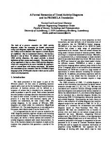
5. Case Study In the sequel we present a SysML activity diagram case study used in order to demonstrate the benefit and usefulness of the proposed formal semantics. Apart from ascribing a rigorous meaning to the informally specified diagrams, formal semantics provides us with an effective technique to uncover design errors that could be missed by intuitive inspection. Furthermore, deriving the formal semantics of activity diagrams allows the application of model transformation and model checking. Practically, the informal description of the behavior captured by the activity diagrams does not enable the automation of the validation process. There is a real need to describe this behavior in a mathematically rigorous way. Thus, our formal framework allows the automation of the validation using existing techniques such as probabilistic model checking. Moreover, it allows reasoning about potential relations between activity diagrams from the behavioral perspective and deriving related mathematical proofs. The SysML activity diagram illustrated in Fig. 13 depicts a hypothetical design of the behavior corresponding to banking operations on an Automated Teller Machine (ATM). The actions therein can be refined using structured activity nodes in order to expand their internal behavior. For instance, the node labeled Withdraw is actually a
4.2.7. Rules for Join. Rules for join are presented in Fig. 12. Rule JOIN -1 and Rule JOIN -2 describe the propagation of a token on the top of the join definition expression, n l : x.Join(M) and the referencing labels. Unlike the merge node, the join traversal requires all references to itself to be marked if the node has 2 (or more) incoming flows. This is stated in the UML standard document under the “join specification” requirement. More precisely, all the subterms l corresponding to a given join node in the AC term, including the definition of join itself, have to be marked. The number of occurrence of l is known and it correspond to the value of x − 1. If so, only one control token propagates to the subsequent subterm M with probability q = 1. Moreover, according to the standard, if we have more than one token on the same incoming edge they are all combined into one. Rule JOIN -2 corresponds to the special case where x = 1. There is no restriction in the standard on the use of a join node with a single incoming edge even though this is qualified as not useful. Rule JOIN -3 shows the possible evolution of n n α l: x.Join(M) to l : x.Join(M� ) , if M −→q M� . 102
Authorized licensed use limited to: CONCORDIA UNIVERSITY LIBRARIES. Downloaded on May 4, 2009 at 09:52 from IEEE Xplore. Restrictions apply.
structured node that calls the activity diagram pictured in Fig. 2. The operational semantics defined earlier allows us performing a compositional assessment of the design. First, the detailed activities are abstracted away and the global behavior is validated, then the refined behavior is assessed. The compositionality and abstraction features allow handling real-world systems without compromising the validation process. For instance, we consider the activity diagram of Fig. 13 and assume Withdraw to be an atomic action d. Moreover, considering the actions a, b, and c as the abbreviations of the actions Authentication, Verify ATM, and Choose account respectively, the corresponding unmarked term A1 , is as follows: A1 = ι � l1: a � l2: Fork(N1 , l12 ) N1 = l3: Merge(l4: b � l5: Fork(N2 , N3 )) N2 = l6: Decision0.9(�g2� l3 , �¬g2� l7: 2.Join(l8: �)) N3 = l9: 2.Join(l10: d � N4 ) N4 = l11: Decision0.3(�g1� N5 , �¬g1� l7 ) N5 = l12: Merge(l13: c � l9 ) The guard g1 denotes the possibility of triggering a new operation if evaluated to true and guard g2 denotes the result of evaluating the status of the connection. Applying the operational rules on the marked A1 , we can derive a run that leads to a deadlock, which means that we reached a configuration where the expression is marked but no progress can be made (no operational rule can be applied). This derivation may reveal a design error in the activity diagram, which is not obvious using only inspection. Even though one may suspect the join2 to cause the deadlock due to the presence of a prior decision node, the deadlock actually occurs in anther node (i.e. node join1). More precisely, the run consists in the execution of action c twice (because the guard g1 is true) and the action b only once (g2 evaluated to false). The deadlocked configuration reached by the derivation run consists in the following marked subterms: M2 = l6: Decision0.9(�g2� l3 , �¬g2� l7: 2.Join(l8: �)) M5 = l12: Merge(l13: c � l9 ) The detailed derivation run is provided in Appendix A. In order to proceed to the validation of functional and nonfunctional requirements, the semantic model (i.e. PTS) has to be entirely derived and then formatted in order to be subjected to probabilistic model checking. Our semantic model presents probabilistic behavior and non-determinism in addition to concurrency, which is the case of Markov Decision Processes (MDP). The latter is supported by various probabilistic model checkers including the Probabilistic Symbolic Model Checker PRISM [24]. Properties to be checked are expressed using the Probabilistic Computation Tree Logic (PCTL) [24]. There are two possible ways to apply probabilistic model checking: either encoding the PTS using the model checker input language or explicitly input the probabilistic transition matrix with the set of states. Due to lack of space, we describe briefly hereafter the second alternative.
Having all reachable states of the semantic model representing all the reachable marking from A1 and the probabilistic transition matrix resulting from the set of probabilistic transitions between states, we have to first process the information into the appropriate accepted file format and then to input both into the model checker. We also input the list of properties to be validated on the model. Finally, properties such as deadlock and reliability can be verified on the model. For instance, the property (1) specifies the eventuality of reaching a deadlock state (with probability P > 0) from any configuration starting at the initial state can be expressed as follows: “init�� ⇒ P > 0 [ F “deadlock�� ]
(1)
Using PRISM model checker, this property returns true, which confirms our previous finding about the presence of a deadlock configuration.
6. Conclusion This paper proposes a formal syntax and semantics for SysML activity diagrams. To the best of our knowledge, this is the first paper that explores this topic. Our main contributions consist in defining a formal dedicated language, namely Activity Calculus (AC), endowed with a formal operational semantics. On the one hand, the syntactic elements of the language are self-descriptive in order to improve its readability. Moreover, it is possible to recover the diagrams from their AC expressions. On the other hand, the semantics provides a rigorous, compositional, and intuitive operational understanding of the behavior captured by the diagram. Furthermore, our approach supports advanced control flows such as unstructured loops, concurrent control flows, and multiple instances of actions. In addition, it handles non well-formed control flows, which allows the use of mixed and nested forks and joins. It is important to notice that although non well-formed activity diagrams are allowed by the standard, many reviewed related work do not support them. Moreover, ascribing a meaning to SysML activity diagram enables the rigorous analysis of the design and the uncovering of design errors early in the development process. As future work, we intend to build on top of the present formalism and to elaborate more on the probabilistic model checking of the SysML activity diagrams. Moreover, we plan to design and implement a practical framework that allows for the automatic derivation of the semantic models and mapping them into the input language accepted by the selected probabilistic model checker.
103
Authorized licensed use limited to: CONCORDIA UNIVERSITY LIBRARIES. Downloaded on May 4, 2009 at 09:52 from IEEE Xplore. Restrictions apply.
References
[14] Y. Jarraya, A. Soeanu, M. Debbabi, and F. Hassa¨ıne, “Automatic Verification and Performance Analysis of Time-Constrained SysML Activity Diagrams,” in the Proceedings of the 14th Annual IEEE International Conference and Workshop on the Engineering of Computer Based Systems(ECBS’07), 26-29 March, Tucson, AZ, U.S.A. IEEE Computer Society, 2007, pp. 515–522.
[1] INCOSE Technical Board, “INCOSE Systems Engineering Handbook - A “What To” Guide for all Systems Engineering Practitioners,” INCOSE, Technical Report TP-2003-016-02, June 2004. [2] Object Management Group, OMG Systems Modeling Language (OMG SysML) Available Specification 1.0, September 2007.
[15] D. Flater, P. A. Martin, and M. L. Crane, “Rendering UML Activity Diagrams as Human-Readable Text,” National Institute of Standards and Technology (NIST), Technical Report NISTIR 7469, November 2007.
[3] C. Bock, “UML 2 Activity Model Support for Systems Engineering Functional Flow Diagrams,” Journal of the International Council on Systems Engineering, vol. 6, no. 4, pp. 123–137, October 2003.
[16] A. Viehl, T. Sch¨anwald, O. Bringmann, and W. Rosenstiel, “Formal Performance Analysis and Simulation of UML/SysML Models for ESL Design,” in the Proceedings of the Conference on Design, Automation and Test in Europe (DATE). European Design and Automation Assoc., 2006, pp. 242–247.
[4] R. W. S. Rodrigues, “Formalising UML Activity Diagrams Using Finite State Processes,” Online Proceedings of UML 2000 Workshop on Dynamic Behaviour in UML Models: Semantic Questions, 2000.
[17] E. B¨orger, A. Cavarra, and E. Riccobene, “An ASM Semantics for UML Activity Diagrams,” in the Proceedings of the 8th International Conference on Algebraic Methodology and Software Technology (AMAST). London, UK: SpringerVerlag, 2000, pp. 293–308.
[5] D. Yang and S. sheng Zhang, “Using π-Calculus to Formalize UML Activity Diagram for Business Process Modeling,” in the 10th International Conference and Workshop on the Engineering of Computer Based Systems (ECBS), 2003, pp. 47–54.
[18] J. P. L´opez-Grao, J. Merseguer, and J. Campos, “From UML Activity Diagrams to Stochastic Petri Nets: Application to Software Performance Engineering,” ACM SIGSOFT Software Engineering Notes, vol. 29, no. 1, pp. 25–36, 2004.
[6] F. Scugl´ık, “Relation Between UML 2 Activity Diagrams and CSP Algebra,” WSEAS Transactions on Computers, vol. 4, no. 10, pp. 1234–1240, 2005.
[19] S. Sarstedt and W. Guttmann, “An ASM Semantics of Token Flow in UML 2 Activity Diagrams,” in Ershov Memorial Conference, ser. Lecture Notes in Computer Science, I. Virbitskaite and A. Voronkov, Eds., vol. 4378. Springer, 2006, pp. 349–362.
[7] N. Tabuchi, N. Sato, and H. Nakamura, “Model-Driven Performance Analysis of UML Design Models Based on Stochastic Process Algebra,” in Proceedings of the European Conference on Model Driven Architecture - Foundations and Applications (ECMDA-FA), ser. Lecture Notes in Computer Science, A. Hartman and D. Kreische, Eds., vol. 3748. Springer, 2005, pp. 41–58.
[20] B. D´enes and R. Heckel, “Rule-Level Verification of Business Process Transformations using CSP,” in Proceedings of the Sixth International Workshop on Graph Transformation and Visual Modeling Techniques (GT-VMT), K. Ehrig and H. Giese, Eds., vol. 6, United Kingdom, May 2007, pp. 13– 27.
[8] H. St¨orrle, “ Semantics of Control-Flow in UML 2.0 Activities,” in IEEE Symposium on Visual Languages and Human-Centric Computing (VL/HCC). Rome, Italy: IEEE Computer Society, 2004, pp. 235–242.
[21] J. H. Hausmann, “Dynamic Meta Modeling: A Semantics Description Technique for Visual Modeling Languages,” Ph.D. dissertation, University Paderborn, 2005.
[9] H. Storrle, “Semantics of Exceptions in UML 2.0 Activities,” Ludwig-Maximilians-Universit¨at M¨unchen, Institut f¨ur Informatik, Tech. Rep. 0403, 2004.
[22] J. Misra and W. R. Cook, “Computation Orchestration,” Software and Systems Modeling, vol. 6, no. 1, pp. 83–110, 2007.
[10] H. St¨orrle, “Semantics and Verification of Data Flow in UML 2.0 Activities,” Electronic Notes in Theoretical Computer Science, vol. 127, no. 4, pp. 35–52, 2005.
[23] E. Best, R. Devillers, and M. Koutny, Petri Net Algebra. New York, NY, USA: Springer-Verlag New York, Inc., 2001.
[11] Object Management Group, OMG Unified Modeling Language: Superstructure 2.1, April 2006.
[24] M. Kwiatkowska, G. Norman, and D. Parker, “Quantitative Analysis with the Probabilistic Model Checker PRISM,” Electronic Notes in Theoretical Computer Science, vol. 153, no. 2, pp. 5–31, 2005.
[12] H. St¨orrle and J. H. Hausmann, “Towards a Formal Semantics of UML 2.0 Activities,” in Software Engineering, ser. LNI, P. Liggesmeyer, K. Pohl, and M. Goedicke, Eds., vol. 64. GI, 2005, pp. 117–128. [13] G. D. Plotkin, “A Structural Approach to Operational Semantics,” University of Aarhus, Technical Report DAIMI FN-19, 1981. 104
Authorized licensed use limited to: CONCORDIA UNIVERSITY LIBRARIES. Downloaded on May 4, 2009 at 09:52 from IEEE Xplore. Restrictions apply.
Appendix 1. Case Study Derivation Run In the sequel, we present a specific derivation run that leads to a deadlocked configuration. The derivation run is presented in Fig. 14 and Fig. 15. This has been obtained by applying the AC operational semantics rules on the term A1 , which corresponds to the initial state of the probabilistic transition system. It represents a single path in the probabilistic transition system corresponding to the semantic model of the activity diagram of Fig. 13. Informally, the deadlock occurs because both join nodes join1 and join2 are waiting for a token that will never be delivered on one of their incoming edges. There is no possible token progress since no rule can be applied.
−→1 ι � l1: a � l2: Fork(l3: Merge(l4: b � l5: Fork( l6: Decision0.9 (�g2� l3 , �¬g2� l7: 2.Join(l8: �)), l9: 2.Join( l10: d � l11: Decision0.3 (�g1� l12: Merge(l13: c � l9 ), �¬g1� l7 )))), l12 ) −→1 ι � l1: a � l2: Fork(l3: Merge(l4: b � l5: Fork( l6: Decision0.9 (�g2� l3 , �¬g2� l7: 2.Join(l8: �)), l9: 2.Join( l10: d � l11: Decision0.3 (�g1� l12: Merge(l13: c � l9 ), �¬g1� l7 )))), l12 ) c
−→1 ι � l1: a � l2: Fork(l3: Merge(l4: b � l5: Fork( l6: Decision0.9 (�g2� l3 , �¬g2� l7: 2.Join(l8: �)), l9: 2.Join( l10: d � l11: Decision0.3 (�g1� l12: Merge(l13: c � l9 ), �¬g1� l7 )))), l12 )
A1 −→1 ι � l1: a � l2: Fork(N1 , l12 )
−→1 ι � l1: a � l2: Fork(l3: Merge(l4: b � l5: Fork( l6: Decision0.9 (�g2� l3 , �¬g2� l7: 2.Join(l8: �)), l9: 2.Join( l10: d � l11: Decision0.3 (�g1� l12: Merge(l13: c � l9 ), �¬g1� l7 )))), l12 )
−→1 ι � l1: a � l2: Fork(N1 , l12 ) −→1 ι � l1: a � l2: Fork(N1 , l12 )
−→1 ι � l1: a � l2: Fork(l3: Merge(l4: b � l5: Fork( l6: Decision0.9 (�g2� l3 , �¬g2� l7: 2.Join(l8: �)), l9: 2.Join( l10: d � l11: Decision0.3 (�g1� l12: Merge(l13: c � l9 ), �¬g1� l7 )))), l12 )
a
−→1 ι � l1: a � l2: Fork(N1 , l12 ) −→1 ι � l1: a � l2: Fork(N1 , l12 )
d
−→1 ι � l1: a � l2: Fork(l3: Merge(l4: b � l5: Fork(N2, N3)), l12 )
−→1 ι � l1: a � l2: Fork(l3: Merge(l4: b � l5: Fork( l6: Decision0.9 (�g2� l3 , �¬g2� l7: 2.Join(l8: �)), l9: 2.Join( l10: d � l11: Decision0.3 (�g1� l12: Merge(l13: c � l9 ), �¬g1� l7 )))), l12 )
−→1 ι � l1: a � l2: Fork(l3: Merge(l4: b � l5: Fork(N2, N3)), l12 ) b
−→0.3 ι � l1: a � l2: Fork(l3: Merge(l4: b � l5: Fork( l6: Decision0.9 (�g2� l3 , �¬g2� l7: 2.Join(l8: �)), l9: 2.Join( l10: d � l11: Decision0.3 (�g1� l12: Merge(l13: c � l9 ), �¬g1� l7 )))), l12 )
−→1 ι � l1: a � l2: Fork(l3: Merge(l4: b � l5: Fork(N2, N3)), l12 ) −→1 ι � l1: a � l2: Fork(l3: Merge(l4: b � l5: Fork(N2, N3)), l12 )
−→1 ι � l1: a � l2: Fork(l3: Merge(l4: b � l5: Fork( l6: Decision0.9 (�g2� l3 , �¬g2� l7: 2.Join(l8: �)), l9: 2.Join( l10: d � l11: Decision0.3 (�g1� l12: Merge(l13: c � l9 ), �¬g1� l7 )))), l12 )
−→0.1 ι � l1: a � l2: Fork(l3: Merge(l4: b � l5: Fork( l6: Decision0.9 (�g2� l3 , �¬g2 = tt� l7: 2.Join(l8: �)), N3)), l12 )
−→1 ι � l1: a � l2: Fork(l3: Merge(l4: b � l5: Fork( l6: Decision0.9 (�g2� l3 , �¬g2� l7: 2.Join(l8: �)), l9: 2.Join( l10: d � l11: Decision0.3 (�g1� l12: Merge(l13: c � l9 ), �¬g1� l7 )))), l12 )
−→1 ι � l1: a � l2: Fork(l3: Merge(l4: b � l5: Fork( l6: Decision0.9 (�g2� l3 , �¬g2� l7: 2.Join(l8: �)), l9: 2.Join( l10: d � l11: Decision0.3 (�g1� l12: Merge(l13: c � l9 ), �¬g1� l7 )))), l12 )
c
−→1 ι � l1: a � l2: Fork(l3: Merge(l4: b � l5: Fork( l6: Decision0.9 (�g2� l3 , �¬g2� l7: 2.Join(l8: �)), l9: 2.Join( l10: d � l11: Decision0.3 (�g1� l12: Merge(l13: c � l9 ), �¬g1� l7 )))), l12 )
Figure 14. The Derivation Run Leading to a Deadlock
Figure 15. The Derivation Run Leading to a Deadlock Continued
105
Authorized licensed use limited to: CONCORDIA UNIVERSITY LIBRARIES. Downloaded on May 4, 2009 at 09:52 from IEEE Xplore. Restrictions apply.