ON THE OPTIMAL CONTROL PROBLEM OF LASER SURFACE ...

c 2010 Institute for Scientific

Computing and Information

INTERNATIONAL JOURNAL OF NUMERICAL ANALYSIS AND MODELING Volume 7, Number 4, Pages 667–680

ON THE OPTIMAL CONTROL PROBLEM OF LASER SURFACE HARDENING NUPUR GUPTA, NEELA NATARAJ AND AMIYA K. PANI Abstract. We discuss an optimal control problem of laser surface hardening of steel which is governed by a dynamical system consisting of a semilinear parabolic equation and an ordinary differential equation with a non differentiable right hand side function f+ . To avoid the numerical and analytic difficulties posed by f+ , it is regularized using a monotone Heaviside function and the regularized problem has been studied in literature. In this article, we establish the convergence of solution of the regularized problem to that of the original problem. The estimates, in terms of the regularized parameter, justify the existence of solution of the original problem. Finally, a numerical experiment is presented to illustrate the effect of regularization parameter on the state and control errors. Key Words. Laser surface hardening of steel, semilinear parabolic equation, ODE with non-differentiable forcing function, regularized Heaviside function, regularised problem, convergence with respect to regularization parameter, numerical experiments.

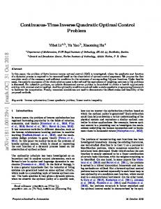
1. Introduction In this paper, we discuss an optimal control problem described by the laser surface hardening of steel. The purpose of surface hardening is to increase the hardness of the boundary layer of a workpiece by rapid heating and subsequent quenching (see Figure 1). The desired hardening effect is achieved as the heat treatment leads to a change in micro structure. A few applications include cutting tools, wheels, driving axles, gears, etc. Let Ω ⊂ R2 , denoting the workpiece, be a convex, bounded domain with piecewise Lipschitz continuous boundary ∂Ω, Q = Ω × I and Σ = ∂Ω × I, where I = (0, T ), T < ∞. Following Leblond and Devaux[7], the evolution of volume fraction of the austenite a(t) for a given temperature evolution θ(t) is described by the initial value problem: (1) (2)

1 [aeq (θ) − a]+ in Q, τ (θ) a(0) = 0 in Ω,

∂t a = f+ (θ, a)

=

where aeq (θ(t)), denoted as aeq (θ) for notational convenience, is the equilibrium volume fraction of austenite and τ is a time constant. The term [aeq (θ) − a]+ = 2000 Mathematics Subject Classification. 65N35, 65N30. The first author would like to acknowledge University Grants of Commission for providing JRF and SRF during her stay in Indian Institute of Technology Bombay. The second and third authors acknowledge the support of the DST Indo-Brazil Project -DST/INT/Brazil/RPO-05/2007 (Grant No. 490795/2007- 2). 667

668

N. GUPTA, N. NATARAJ AND A. PANI

Figure 1. Laser Hardening Process (aeq (θ) − a)H(aeq (θ) − a), where H is the Heaviside function  1 s>1 H(s) = 0 s ≤ 0, denotes the non-negative part of aeq (θ) − a, that is, (aeq (θ) − a) + |aeq (θ) − a| . [aeq (θ) − a]+ = 2 Neglecting the mechanical effects and using the Fourier law of heat conduction, the temperature evolution can be obtained by solving the following energy balance equation: (3)

ρcp ∂t θ − K △ θ

=

−ρL∂t a + αu in Q,

(4)

θ(0) = θ0 in Ω, ∂θ (5) = 0 on Σ, ∂n where the density ρ, the heat capacity cp , the thermal conductivity K and the latent heat L are assumed to be positive constants. Further, θ0 denotes the initial temperature. The term u(t)α(x, t) describes the volumetric heat source due to laser radiation and the laser energy u(t) is a time dependent control variable. Since the main cooling effect is a self-cooling of the workpiece, a homogeneous Neumann condition is assumed on the boundary. To maintain the quality of the workpiece surface, it is important to avoid the melting of the surface. In the case of laser hardening, it is a quite delicate problem to obtain parameters that avoid melting but nevertheless lead to the right amount of hardening. Mathematically, this corresponds to an optimal control problem in which we minimize the cost functional defined by: Z Z Z Z β2 T β3 T 2 β1 (6) J(θ, a, u) = |a(T ) − ad |2 dx + [θ − θm ]2+ dxds + |u| ds 2 Ω 2 0 Ω 2 0 (7) subject to (1) − (5) in the set of admissible controls Uad , where Uad = {v ∈ U : kvkU ≤ M, for fixed positive M } with U = L2 (I), β1 , β2 and β3 are positive constants and ad is the given desired fraction of the austenite. The second term in (6) is a penalizing term that penalizes the temperature below the melting temperature θm . The mathematical model for the laser surface hardening of steel has been studied in [4] and [7]. For an extensive survey on mathematical models for laser material

ON THE OPTIMAL CONTROL PROBLEM OF LASER SURFACE HARDENING

669

treatments, we refer to [9]. In this article, we follow the Leblond-Devaux model [7]. In [1], [4], the mathematical model for the laser hardening problem is discussed and results on existence, regularity and stability are derived. In [3], the authors have investigated two different methods of surface hardening: laser and induction hardening and then for numerical approximation, they have applied finite volume method for space discretization and finite difference for temporal discetization of the regularised problem. In [5], the optimal control problem is analyzed and related error estimates for the regularised state system are derived using proper orthogonal decomposition (POD) Galerkin method. In [12], a nonlinear conjugate gradient method has been used to solve the optimal control problem and a finite element method has been used for the purpose of space discretization. Recently in [10], the authors have derived a priori error estimates for the regularized laser surface hardening problem. The presence of the term [aeq −a]+ in the right hand side of (1) creates a problem in developing analytical results and finding numerical solution. In order to overcome 1 this difficulty, the function f+ = τ (θ) [aeq − a]+ is regularized using a regularized Heaviside function in literature (see [3]-[6], [12]). Although the numerical schemes in [3]-[6] and [12] are discretizations of the regularized problem, there are hardly any convergence results available which establish the fact that the solution of the regularized problem converges to that of the original problem as the regularization parameter ǫ tends to zero. In this paper, it is shown that the error between the solution of regularized problem and that of the original problem is of order O(ǫ) and a convergence analysis for the regularized laser surface hardening of steel problem is discussed. The outline of this paper is as follows. In Section 2, we describe the regularized optimal control problem of laser surface hardening of steel and its weak formulation with results of existence and uniqueness of solution, which are already available in the literature. A stability result for the temperature is also established. In Section 3, the existence of a unique solution for (1)-(5) is proved for a fixed control u and then the convergence of the solution of the regularized problem to that of the original problem is proved. Finally, Section 4 gives numerical results, which justifies the theoretical results obtained in Section 3.

2. The Regularized Problem In this section, we first present a regularized problem and recall some related results on existence, uniqueness and regularity. With ǫ > 0 as regularization parameter, we replace the Heaviside function by a regularized function Hǫ ∈ C 1,1 (R), where Hǫ is a monotone approximation of the Heaviside function satisfying Hǫ (x) = 0 for x ≤ 0. Thus, we arrive at the following regularized problem: (1) (2)

min J(θǫ , aǫ , uǫ ) subject to

uǫ ∈Uad

∂t aǫ

= fǫ (θǫ , aǫ ) in Q,

(3) (4)

aǫ (0) = 0 in Ω, ρcp ∂t θǫ − K △ θǫ = −ρL∂t aǫ + αuǫ in Q,

(5)

θǫ (0) = θ0 in Ω, ∂θǫ = 0 on Σ, ∂n

(6)

670

N. GUPTA, N. NATARAJ AND A. PANI

where β1 2

J(θǫ , aǫ , uǫ ) =

Z

|aǫ (T ) − ad |2 dx +

Ω

and fǫ (θǫ , aǫ ) =

β2 2

Z

T 0

Z

Ω

[θǫ − θm ]2+ dxds +

β3 2

Z

T

|uǫ |2 ds,

0

1 (aeq (θǫ ) − aǫ )Hǫ (aeq (θǫ ) − aǫ ). τ (θǫ )

We now make the following assumptions [5]: (A1) aeq (s) ∈ (0, 1) for all s ∈ R and kaeq kC 1 (R) ≤ ca ; (A2) 0 < τ ≤ τ (s) ≤ τ¯ for all s ∈ R and kτ kC 1 (R) ≤ cτ ; (A3) θ0 ∈ H 1 (Ω), θ0 ≤ θm a.e. in Ω, where the constant θm > 0 denotes the melting temperature of the steel; (A4) α ∈ L∞ (I, L∞ (Ω)); (A5) u ∈ L2 (I); (A6) ad ∈ L∞ (Ω) with 0 ≤ ad ≤ 1 a.e. in Ω.

1.5

1.5 Regularized Heaviside Function

Heaviside Function

1

1

0.5

0.5

0

0

−0.5 −1

−0.5

0

0.5

1

−0.5 −1

−0.5

0

0.5

1

Figure 2. Regularized Heaviside(Hǫ ) and Heaviside(H) Functions Below, we discuss the weak formulation corresponding to the regularized problem (1)-(6). Let X = {v ∈ L2 (I; H 1 (Ω)) : vt ∈ L2 (I; H −1 (Ω))}. The Hilbert space H 1 (Ω) and its dual H −1 (Ω) build a Gelfand triple H 1 (Ω) ֒→ L2 (Ω) ֒→ H −1 (Ω). The duality pairing between H 1 (Ω) and H −1 (Ω) is denoted by < ·, · >= < ·, · >H −1 (Ω)×H 1 (Ω) . Let the inner product and norm in L2 (I) be denoted by (·, ·)L2 (I) and k · kL2 (I) , respectively. Now the weak formulation corresponding to the regularized problem (1)-(6) is given by (7) (8) (9) (10) (11)

min J(θǫ , aǫ , uǫ ) subject to

uǫ ∈Uad

(∂t aǫ , w) = aǫ (0) = ρcp (∂t θǫ , v) + K(∇θǫ , ∇v) = θǫ (0) =

(fǫ (θǫ , aǫ ), w), 0, −ρL(∂t aǫ , v) + (αuǫ , v), θ0 ,

ON THE OPTIMAL CONTROL PROBLEM OF LASER SURFACE HARDENING

671

1 for all (w, v) ∈ L2 (Ω)×H 1 (Ω), a.e. in I, where fǫ (θ, a) = τ (θ) (aeq (θ)−a)Hǫ (aeq (θ)− a). The following theorem ([12], Theorem 2.1) ensures the existence and uniqueness of solution of the regularized problem (8)-(11).

Theorem 2.1. Suppose that assumptions (A1)-(A6) are satisfied. Then, for a given uǫ ∈ Uad the system (8)-(11) has a unique solution (θǫ , aǫ ) ∈ H 1,1 (Q) × W 1,∞ (I; L∞ (Ω)), where H 1,1 = L2 (I; H 1 (Ω)) ∩ H 1 (I; L2 (Ω)). Moreover, aǫ satisfies 0 ≤ aǫ < 1 a.e. in Q. Remark 2.1. Due to (A1)-(A2) and nature of the regularized Heaviside function, there exists a constant cf > 0 independent of θǫ and aǫ such that max(kfǫ (θǫ , aǫ )kL∞ (Q) , k

∂fǫ ∂fǫ (θǫ , aǫ )kL∞ (Q) , k (θǫ , aǫ )kL∞ (Q) ) ≤ cf ∂a ∂θ

for all (θǫ , aǫ ) ∈ L2 (Q) × L∞ (Q). The existence of a global solution to the optimal control problem (1)-(6) is guaranteed by the following theorem ([12], Theorem 2.3). Theorem 2.2. Suppose that the assumptions (A1)-(A6) are satisfied. Then the optimal control problem (1)-(6) has at least one(global) solution. The next lemma shows the stability result for the temperature θǫ when aǫ ∈ W 1,∞ (I, L∞ (Ω)). Lemma 2.1. Suppose that the assumptions (A1)-(A6) are satisfied. Then, for a fixed uǫ ∈ Uad , the first component of the solution (θǫ , aǫ ) ∈ H 1,1 ×W 1,∞ (I, L∞ (Ω)) of (4)-(6), satisfies kθǫ kL∞ (I,H 1 (Ω))

≤

C,

where C > 0 is a finite constant. Proof. Set v = θǫ in (10) to obtain ρcp d kθǫ k2 + k∇θǫ k2 = −ρL(∂t aǫ , θǫ ) + (αuǫ , θǫ ) 2 dt Integrating from 0 to t, using Cauchy-Schwarz and Young’s inequality, we find that  Z t Z t kθǫ (t)k2 + k∇θǫ k2 dt ≤ C kθ0 k2 + (k∂t aǫ k2 + |uǫ |2 )dt 0 0  Z t (12) + kθǫ k2 dt . 0

Using Gronwall’s Lemma, it follows that   Z t (13) kθǫ (t)k2 ≤ C kθ0 k2 + (k∂t aǫ k2 + |uǫ |2 )dt . 0

Now, multiply (4) with ∂t θǫ , integrate over Ω and use Cauchy-Schwarz and Young’s inequality to obtain   1 d ρcp ρcp k∂t θǫ k2 + k∇θǫ k2 ≤ C k∂t aǫ k2 + |uǫ |2 + k∂t θǫ k2 . 2 dt 2

672

N. GUPTA, N. NATARAJ AND A. PANI

Hence, integrating from 0 to t, we arrive at    Z t Z t (14) k∂t θǫ k2 dt + k∇θǫ (t)k2 ≤ C k∇θ0 k2 + k∂t aǫ k2 + |uǫ |2 dt . 0

0

1,∞

∞

Since aǫ ∈ W (I, L (Ω)) and uǫ ∈ Uad , using (A3), (13) and (14) we obtain the desired result. This completes the proof.  3. Convergence Analysis Below, we first present the weak formulation corresponding to the (6)-(7): (1)

min J(θ, a, u) subject to

u∈Uad

(2) (3)

(∂t a, w) = a(0) =

(4) (5)

ρcp (∂t θ, v) + K(∇θ, ∇v) = θ(0) =

(f+ (θ, a), w), 0, −ρL(∂t a, v) + (αu, v), θ0 ,

1 for all (w, v) ∈ L2 (Ω)×H 1 (Ω) a.e. in I, where f+ (θ, a) = τ (θ) (aeq (θ)−a)H(aeq (θ)− a). In this section, we prove that for a fixed control u ∈ Uad , solution to the problem (8)-(11) converges to the solution of (2)-(5). Then we discuss the existence of solution of the optimal control problem and finally, convergence of the regularized problem as the regularized parameter tends to zero.

Theorem 3.1. Let the assumptions (A1)-(A6) hold true. Then, for a fixed u ∈ Uad , there exists a unique solution (θ, a) to (2)-(5) and for all ǫ ∈ (0, 1), t ∈ I, the following estimate holds: (6)

ka(t) − aǫ (t)k + kθ(t) − θǫ (t)k ≤ C(Ω, T )ǫ,

where C(Ω, T ) is a positive constant and (θǫ , aǫ ) is the solution to the problem (8)-(11) for the fixed u ∈ Uad . Proof. From Theorem 2.1, the sequence {(θǫ , aǫ )} is uniformly bounded in H 1,1 × W 1,∞ (I, L∞ (Ω)), and from Lemma 2.1, the sequence {θǫ } is uniformly bounded in L∞ (I, H 1 (Ω)). Therefore, using weak and weak∗ compactness arguments and H 1 (Ω) being compactly imbedded in L2 (Ω) , we obtain (7)

θǫ

−→ θ strongly in C(I, L2 (Ω)),

(8)

θǫ

−→ θ weakly in H 1,1 ,

(9)

aǫ

−→ a weak∗ in W 1,∞ (I, L∞ (Ω)).

For θ ∈ C(I, L2 (Ω)) and f+ being globally Lipschitz continuous, (2)-(3) has a unique solution a (say). Now subtracting (8) from (2), putting w = a − aǫ and using Cauchy-Schwarz’s and Young’s inequality, we obtain d ka − aǫ k2 ≤ kfǫ (θǫ , aǫ ) − f+ (θ, a)k2 + ka − aǫ k2 . dt Now integrating from 0 to t, it follows that Z t  Z t (10) k(a − aǫ )(t)k2 ≤ C kfǫ (θǫ , aǫ ) − f+ (θ, a)k2 dt + ka − aǫ k2 dt . 0

0

Note that using triangle inequality, we arrive at   (11) kfǫ (θǫ , aǫ ) − f+ (θ, a)k2 ≤ C kfǫ (θǫ , aǫ ) − fǫ (θ, a)k2 + kfǫ (θ, a) − f+ (θ, a)k2 .

ON THE OPTIMAL CONTROL PROBLEM OF LASER SURFACE HARDENING

673

For the first term on the right hand side of (11), use Remark 2.1 to obtain   (12) kfǫ (θǫ , aǫ ) − fǫ (θ, a)k2 ≤ C kθǫ − θk2 + kaǫ − ak2 . For the second term on the right hand side of (11), using the assumption (A2), we find that kfǫ (θ, a) − f+ (θ, a)k2 1 ≤ k(aeq (θ) − a)H(aeq (θ) − a) − (aeq (θ) − a)Hǫ (aeq (θ) − a)k2 τ Z 1 (aeq (θ) − a)2 (H(aeq (θ) − a) − Hǫ (aeq (θ) − a))2 dx. = τ Ω Let Ω1 = {x ∈SΩ : aeq − a ≤ 0 or aeq − a ≥ ǫ} and Ω2 = {x ∈ Ω : 0 < aeq − a < ǫ}. Since Ω = Ω1 Ω2 , we arrive at kfǫ (θ, a) − f+ (θ, a)k2 Z 1 ≤ (aeq (θ) − a)2 (H(aeq (θ) − a) − Hǫ (aeq (θ) − a))2 dx τ Ω1 Z 1 (aeq (θ) − a)2 (H(aeq (θ) − a) − Hǫ (aeq (θ) − a))2 dx. + τ Ω2

From Figure 2, it follows that (13)

kfǫ (θ, a) − f+ (θ, a)k2

1 τ

≤

Z

ǫ2 dx ≤ C(Ω)ǫ2 .

Ω2

Substituting (13) in (11), we obtain (14)

  2 2 2 kfǫ (θǫ , aǫ ) − f+ (θ, a)k ≤ C kθǫ − θk + kaǫ − ak + ǫ . 2

Substituting (14) in (10), we find using Gronwall’s lemma that Z t  2 2 2 ka − aǫ k ≤ C(Ω, T ) kθ − θǫ k dt + ǫ 0

Using (7), we arrive at (15)

aǫ −→ a strongly in L∞ (I, L2 (Ω)).

From (14), using (7), (15), we obtain as ǫ −→ 0 (16)

fǫ (θǫ , aǫ ) −→ f+ (θ, a).

Now letting ǫ → 0 in (8)-(11) and using (7)-(9), (15), (16), we obtain the existence of solution of (2)-(5). For proving uniqueness we proceed as follows. If possible, let (θ1 , a1 ) and (θ2 , a2 ) be two different solutions of (2)-(5). Therefore, from (4), we obtain (17) ρcp (∂t (θ1 − θ2 ), v) + K(∇(θ1 − θ2 ), ∇v) = −ρL(f+ (θ1 , a1 ) − f+ (θ2 , a2 ), v). Setting v = θ1 − θ2 in (17), use Young’s inequality to obtain   d 2 2 2 2 (18) kθ1 − θ2 k + k∇(θ1 − θ2 )k ≤ C kf+ (θ1 , a1 ) − f+ (θ2 , a2 )k + kθ1 − θ2 k dt Similarly from (2), we arrive at   d (19) ka1 − a2 k2 ≤ C kf+ (θ1 , a1 ) − f+ (θ2 , a2 )k2 + ka1 − a2 k2 . dt

674

N. GUPTA, N. NATARAJ AND A. PANI

Adding (18) and (19), using Lipschitz continuity of the functions aeq , f+ , integrating from 0 to T and finally using Gronwall’s lemma, we obtain kθ1 − θ2 k2 + ka1 − a2 k2

≤

0,

which proves uniqueness. To prove (6), subtract (8) from (2), put w = a − aǫ , use Cauchy-Schwarz and Young’s inequality to find that   d 2 2 2 (20) ka − aǫ k ≤ kf+ (θ, a) − fǫ (θǫ , aǫ )k + ka − aǫ k . dt Now integrating from 0 to t, we obtain Z t  Z t 2 2 2 (21) ka(t) − aǫ (t)k ≤ kf+ (θ, a) − fǫ (θǫ , aǫ )k dt + ka − aǫ k dt . 0

0

Similarly, for a fixed u ∈ Uad and uǫ = u, subtract (10) from (4), substitute v = θ − θǫ , integrate from 0 to t and use (20) to arrive at Z t kθ(t) − θǫ (t)k2 + k∇(θ − θǫ )k2 dt 0 Z t Z t ≤ C kf+ (θ, a) − fǫ (θǫ , aǫ )k2 dt + ka − aǫ k2 dt 0 0  Z t 2 (22) + kθ − θǫ k dt . 0

Adding (21) and (22), we find that ka(t) − aǫ (t)k2

(23)

+ kθ(t) − θǫ (t)k2 Z t Z t ≤ C kf+ (θ, a) − fǫ (θǫ , aǫ )k2 dt + ka − aǫ k2 dt 0 0  Z t + kθ − θǫ k2 dt . 0

Using (14), we now obtain 2

ka(t) − aǫ (t)k + kθ(t) − θǫ (t)k

2

≤

  Z t 2 2 2 C(Ω, T ) ǫ + (kθ − θǫ k + ka − aǫ k )dt . 0

Using Gronwall’s lemma, we arrive at (24)

ka(t) − aǫ (t)k + kθ(t) − θǫ (t)k

≤

C(Ω, T )ǫ.

This completes the proof.



Remark 3.1. Using (24) in (22), we obtain kθ − θǫ kL2 (I,H 1 (Ω))

≤

C(Ω, T )ǫ.

Below, we discuss existence of solution to the optimal control problem (1)-(5). For u∗ ∈ Uad , let (θ∗ , a∗ ) be a solution of (2)-(5). Now, the existence of a unique solution to the state equations (2)-(5) ensures the existence of a control-to-state mapping u 7→ (θ, a) = (θ(u), a(u)) through (2)-(5). By means of this mapping, we introduce the reduced cost functional j : Uad −→ R as (25)

j(u) = J(θ(u), a(u), u).

ON THE OPTIMAL CONTROL PROBLEM OF LASER SURFACE HARDENING

675

Then the optimal control problem can be equivalently reformulated as (26)

min j(u) subject to the dynamical system (2) − (5).

u∈Uad

Theorem 3.2. (1)-(5) has at least one solution (θ∗ , a∗ , u∗ ) ∈ X × X × Uad . Proof. Let l = inf j(u) and {un }n∈N ⊂ Uad be a minimizing sequence such that u∈Uad

(27)

j(un ) −→ l in R.

Since Uad is bounded, the sequence {un } is bounded uniformly in L2 (I). Therefore, one can extract a subsequence {un }(say), such that un −→ u∗ weakly in L2 (I). Since the admissible space Uad is a closed and convex subset of L2 (I), it is weakly closed in L2 (I) and hence, u∗ ∈ Uad . Corresponding to each un , we obtain (θn , an ) ∈ H 1,1 × W 1,∞ (I, L∞ (Ω)) satisfying (2)-(5), and θn ∈ L∞ (I, H 1 (Ω)). Therefore, we can extract a subsequence {(θn , an )}( again say) such that θn θn

−→ θ∗ weakly in H 1,1 −→ θ∗ strongly in C(I, L2 (Ω))

an

−→ a∗ weak∗ in W 1,∞ (I, L∞ (Ω))

an

−→ a∗ strongly in L∞ (I, L2 (Ω)).

Now letting n → ∞ in the following problem (∂t an , w) = an (0) = ρcp (∂t θn , v) + K(∇θn , ∇v) = θn (0) =

(f+ (θn , an ), w) ∀w ∈ V, 0 −ρL(∂t an , v) + (αun , v) ∀v ∈ V, θ0 ,

we obtain (θ∗ , a∗ ) as a unique solution of (2)-(5) corresponding to the control u∗ ∈ Uad and hence, (θ∗ , a∗ , u∗ ) is an admissible solution. Now we claim that it is an optimal solution. Since j is lower semi-continuous, j(u∗ ) ≤ lim inf j(un ) n→∞

and using (27), we obtain j(u∗ ) ≤ l. Thus, u∗ is a minimizer of the cost functional j and (θ∗ , a∗ , u∗ ) is an optimal solution. This completes the rest of the proof.  3.1. Convergence of the Control Function. Theorem 3.3. Let u∗ǫ be the optimal control of (7)-(11), for 0 < ǫ < 1. Then, lim u∗ǫ = u∗ exists in L2 (I) and u∗ is an optimal control of (1)-(5). ǫ→0

Proof: Since u∗ǫ is an optimal control, we obtain ku∗ǫ kL2 (I) ≤ M, 0 < ǫ < 1, that is, {u∗ǫ }0