identification algorithm, POEIV-MOESP, is proposed for power system damping control. Under closed-loop condition and based on wide-area measurements, ...
Online Recursive Closed-Loop State Space Model Identification for Damping Control Hua Ye, Yutian Liu, Senior Member, IEEE School of Electrical Engineering, Shandong University Jinan, China {yehua, liuyt}@sdu.edu.cn Abstract—An online recursive closed-1oop state space model identification algorithm, POEIV-MOESP, is proposed for power system damping control. Under closed-loop condition and based on wide-area measurements, reduced order state space model of the system which contains dominant low frequency oscillation modes is firstly identified by the algorithm, then recursively updated by EIV-PAST algorithm and RLS method. The model identification algorithm combing with a model predictive control is tested on the New England 10-machine 39-bus system, and the effectiveness of both the model identification algorithm and the controller are demonstrated.
II.
CLOSED-LOOP SUBSPACE IDENTIFICATION ALGORITHM
A. Modeling of a power system Around a stable operating point, a power system can be described using a closed-loop structure showed in Fig. 1. wk u� k
rk
Keywords-dmping control; closed-loop identification; subspace identification; recursive estimaiton
I.
INTRODUCTION
Modeling a power system is the basis and premise of control strategy design for low frequency oscillations (LFO) damping. In an interconnected power system, there are usually hundreds of generators. Thus, it is difficult to obtain the mathematical model of such a system which is of very high order. Presently, model order reduction (MOR) methods have been proposed to design damping controllers for large scale systems, in which transfer functions or state-space models with reduced orders are obtained by open-loop identification using system dynamic responses [1–2]. However, it is difficult for the MOR-based controllers to adapt to large changes in system operating conditions because of the fixed parameters they have employed. To overcome inherent shortcomings of conventional damping controllers, adaptive controllers have been developed for robustness enhancement [3]. It is the reduced order transfer function, not the state-space model, can be directly derived from RLS [3] and the popular Prony algorithm [1], where the latter is more convenient for control design. Recently, subspace identification algorithms have been proposed for power system LFO analysis [4–5]. Compared with the prediction error method (PEM), there is no underlying nonlinear iterative optimization and related problems such as convergence, local minima, and high computational burden. In this paper, the subspace model identification method is extended from LFO analysis to damping. The contributions are mainly in two folds. The first is closed-loop state space model identification, and the other is online updating system model and adjusting control inputs. The proposed model identification algorithm combing with a model predictive controller (MPC) [6] is tested on the New England 10-machines 39-bus system.
fk
uk
vk
xk +1 = Ak xk + Bk u� k + f k y� k = C k xk + d k
y� k
yk
Fig. 1 Closed-loop structure of a system.
The system excluding the controller can be written as
xk +1 = Ak xk + Bk u� k + f k , uk = u� k + wk y� k = C k xk + d k , yk = y� k + v k n×n
n×m
(1)
l×n
and Ck ∈R are system matrices. where Ak ∈R , Bk ∈R xk, ũk and ỹk ∈Rl×1 denote system state, control input and plant output, while uk and yk are measured input and output, respectively. fk is an exogenous perturbation vector, including random load switching, and set-point and topology changes actuated by faults, line and generator tripping, and load shedding [4]. rk ∈Rm×1 is the measurable reference. dk is the output disturbance; wk and vk are input and output measurement noises, respectively. wk and vk are assumed to be zero-mean, white noises. B. POEIV-MOESP algorithm The essential elements of the past output errors in variables-MIMO error state space (POEIV-MOESP) algorithm are introduced as follows. Readers are referred to [7–8] for the detailed information and proofs.
i) Collect a sequence of input vector (u1, u2, …, uk) and output vector (y1, y2, …, yk) and build block Hankel matrices as follows
U k ,s, N
⎡ uk ⎢u = ⎢ k +1 ⎢ # ⎢ ⎣ uk + s −1
This work was supported by the Natural Science Foundation of China under Grant 50877044 and in partly by the National High Technology Research and Development of China under Grant 2009AA05Z213.
978-1-4244-4813-5/10/$25.00 ©2010 IEEE
uk + N −1 ⎤ " uk + N ⎥⎥ ⎥ % # ⎥ " uk + s + N − 2 ⎦
uk +1 " uk + 2 # uk + s
(2)
U k + s,s, N
⎡ uk + s ⎢u = ⎢ k + s +1 ⎢ # ⎢ ⎣ uk + 2 s −1
uk + s + N −1 ⎤ " uk + s + N ⎥⎥ ⎥ % # ⎥ " uk + 2 s + N − 2 ⎦
uk + s +1 "
φup (k + 1) = [ukT+ N
" ukT+ s + N −1 ]T
uk + s + 2
φyp (k + 1) = [ ykT+ N
"
# uk + 2 s
(3)
where s and N indicate the number of block rows and columns of the block Hankel matrices, respectively. Similarly, Yk,s,N and Yk+s,s,N are also constructed. ii) Select [(Uk,s,N) T (Yk,s,N) T] as an instrumental matrix to eliminate noises fk, wk and vk, then the subspace spanned by the column of extended observability matrix Γs can be derived from following projection using the RQ factorization ⎡U k + s , s , N U kT, s , N U k + s , s , N YkT, s , N ⎤ ⎡ R11N 0 ⎤ ⎡Q1N ⎤ = ⎢ ⎥ ⎢ N T T N ⎥⎢ N⎥ (4) ⎣⎢ Yk + s , s , N U k , s , N Yk + s , s , N Yk , s , N ⎦⎥ ⎣ R21 R22 ⎦ ⎣Q2 ⎦
then
lim
N →∞
then
ykT+ s + N −1 ]T
φuf (k + 1) = [ukT+ s + N
" ukT+ 2 s + N −1 ]T
φyf (k + 1) = [ ykT+ s + N
"
feeding
ykT+ 2 s + N −1 ]T
(8)
T φyf (k + 1) − Hˆ (k )φuf (k + 1) and [φup (k + 1)
φTyp (k + 1)] directly to the EIV-PAST algorithm to recursively update Γs [8], where Hs is a Toplitz matrix defined as 0 ⎡ D ⎢ CB D Hs = ⎢ ⎢ # # ⎢ s −2 s −3 CA B CA B ⎣
" 0⎤ " 0 ⎥⎥ % 0⎥ ⎥ " D⎦
(9)
According to the updated Γs, matrices Ak and C k can be
1 N
R22N = lim
N →∞
1 N
Γ s X k + s , N [U kT, s , N YkT, s , N ] ( Q2N )
T
(5)
Eq. (5) shows that subspace spanned by the column of R22N lies in the column space of Γs, which is defined as Γs=[CT (CA)T … (CAn–1)T]T. iii) Calculate the singular value decomposition (SVD) of the projection matrix R22N R = USV = [U1 N 22
T
⎡S U2 ] ⎢ 1 ⎣0
0 ⎤ ⎡V1T ⎤ ⎢ ⎥ S 2 ⎥⎦ ⎣V2T ⎦
(6)
(7)
where (⋅) denotes the Moore-Penrose pseudo-inverse. Γ s and †
Γ s are obtained by removing the last and the first l rows of Γs, respectively. The matrix Ck can be determined from the first l rows of Γs.
v) Select an appropriate instrumental matrix to eliminate noises and then compute matrix Bk using the least square method from the input-output vector. III.
Once the discrete system model {Ak, Bk, Ck} is updated, it can be converted into a continuous model {A, B, C} by using a bilinear (Tustin) approximation. Then frequencies and damping ratios corresponding to eigenvalues of A can be accordingly computed. IV.
iv) Calculate Γs and compute Ak and Ck Γ s = U1 S11/ 2 , Ak = Γ†s Γ s
easily computed, then matrix Bk can be accordingly updated by the RLS method.
RECURSIVE UPDATING OF SYSTEM MATRICES
The state-space model identified by the POEIV-MOESP algorithm should be updated online so as to adapt to system variations. In the algorithm, time complexity is the most timeconsuming step. To overcome this difficulty, the extended instrumental variable-projection approximation subspace tracking (EIV-PAST) algorithm proposed in [9] is adopted. The basic idea is to treat the signal subspace-tracking problem as the solution of an unconstrained minimization task. Furthermore, a projection approximation reduces the minimization to the well-known exponentially weighted least squares problem. At time instant k =k+2s+N–2, define following vectors using the new arriving input and output samples
APPLICATION TO POWER SYSTEM DAMPING CONTROL
A. Aspects on applying RPO-MOESP to damping control Following aspects should be carefully considered for applying the recursive PO-MOESP (RPO-MOESP) algorithm to power system damping control. 1) Choice of excitation signal: The RPO-MOESP algorithm requires persistent excitation. That is to say that, the reference rk and input ũk are sufficiently rich to excite dynamics of the system, so that identification can take place [7]. For power system damping control, dynamics in the low frequency oscillation band are mostly expected to be excited. Therefore, an ideal band-pass signal together with a Hamming window is used to inject into power system to excite dominant low frequency oscillation modes. In time domain, it is formulated as ⎡ sin ( 2π f h ( t − T0 ) ) − sin ( 2π f l ( t − T0 ) ) ⎤ Pd ( t ) = P0 ⋅ w ( t ) ⋅ ⎢ ⎥ π ( t − T0 ) ⎢⎣ ⎥⎦ (10) where, [fl, fh] is the frequency band; T0 = T/2, T is the period of injected excitation signal; P0 is the power coefficient corresponding to the amplitude of its frequency response. The maximum of the signal in time domain is 2P0(fh – fl). The Hamming window function w(t)is used to reduce ripples. 2) Scale change of sampled data: In practice, signals of a widely differing physical significance, such as power flow in a tie-line (MW), shaft speed (rad/s) and angle shift (deg.) between different areas, etc. may be involved simultaneously in inputs of the RPO-MOESP algorithm. Since the proposed algorithm is sensitive to scaling of the inputs and outputs, it
will suffer from a scaling problem. Therefore, choice of appropriate scaling factors for the algorithm will help improve accuracy of model identification. B. Flowchart of applng RPO-MOESP to damping control Injecting excitation signal Pd(t) into reference input of the voltage regulator
Sample and scale uk and yk k ≥ 2s+N–1?
k = 2s+N–1?
Identify system model {Ak, Bk, Ck} using POEIVMOESP algorithm
k←k+1
No
Yes No
Update system model using RPOEIV-MOESP algorithm
Controller design and online updating the control action ũk
Fig. 3 The 10-machine 39-bus New England test system.
Controller design and updating
0.12
ũk ←0 Excitation signal Pd (p.u.)
Yes
Model identification
Apply control action
Fig.2 Flow chart of application of RPO-MOESP algorithm to damping control
The flow chart of applying the online recursive closedloop state-space model identification algorithm, i.e., RPOMOESP to power system damping control is shown in Fig. 2. It consists two parts. The first part accomplishes identification and updating system reduced model. Based on the identified model, the second part designs wide-area damping controller using such as optimal control, and adaptive control, etc.
The 10-machine 39-bus New England system is used to demonstrate the effectiveness of the proposed closed-loop model identification algorithm. The configuration of the test system is shown in Fig. 3. All generators are represented by the double-axis model equipped with IEEE type DC1A excitation systems and PSSs. Parameters for generators and exciters are derived from data provided by the Power System Toolbox (PST). Parameters for PSSs can be found in [8]. Loads are represented by constant impedances. Under normal operating condition, tie-line power flow is 494MW. Small signal stability analysis shows that the system has an inter-area oscillation mode, wherein the equivalent generator G1 swings against other generators. Frequency of the mode is 0.55Hz, and the damping ratio is 6.68%. Here, an adaptive model predictive controller (MPC) as a damping controller is designed and supplemented to excitation system of generator G7 in the coherent generator group (G4, G5, G6, G7). Δω7–1, ΔP4–5, ΔP16–17, and ΔP15–16 are selected as widearea feedback signals through controllability and observability analysis. Excitation signal as showed in Fig. 4 is injected to Vs periodically. Then control input and those feedback signals are sampled, scaled, and sent to RPOEIV-MOESP algorithm to identify system model. At last, control input ũk7 are calculated and updated.
0
2
4
6
8
10
Time (s)
Fig. 4 Time domain response of the excitation signal Pd. 1.1 Frequency f (Hz)
CASE STUDIES
0.04
-0.04 0
Original
0.9
Identified by RPI Identified by RPOEIV
0.7 0.5 0.3 20
25
30
35
40
45
50
Time (s) (a)
100 Damping ratio ζ (%)
V.
0.08
Original
80
Identified by RPI Identified by RPOEIV
60 40 20 0 20
25
30
35
40
45
50
Time (s) (b)
Fig. 5 Identified frequencies and damping ratios: (a) Frequency f. (b) Damping ratio ζ.
Fig. 5 shows the identified frequencies and damping ratios for system following a three-phase-to-ground short circuit fault occurring at the middle of line 3–18 at t=28s and cleared in 0.06s without line tripping. The line is selected as it sits near the transmission section {16–15, 16–17}. In the figure, dashed lines denote frequency and damping ratio via small signal stability analysis, while dash-dot and solid lines are those identified online by RPI-MOESP used in [11] and RPOEIV-MOESP proposed in this paper, respectively.
It can be seen from Fig. 5 that there are sharp changes in identified frequencies and damping ratios soon after the disturbance. After t=31s, the frequency identified by RPOEIVMOESP almost coincides with the original value. However, errors between identified damping ratio and its original value are quite large. The phenomenon may be explained as follows. Strictly speaking, the actual responses of power system often contain non-stationary condition. Especially, ringdowns are included during and soon after a large disturbance. In general, as system responses to a large disturbance contain more modal energy than system under normal operating condition, identified model is improved and more accurate frequency estimation is obtained. However, due to sharp change of system responses, large estimate error in identified damping ratio appears. In fact, the situation displayed in this figure that frequency estimate is much more accurate than damping estimate, is also found in performance tests for other identification algorithms [5]. However, with regards to the RPI-MOESP algorithm, estimate errors in both frequency and damping ratio are large. Deviation of relative rotor speed Δω 7-1 (p.u.)
-3
6
x 10
Measured
4
Estimated by RPOEIV
2 0
VI.
CONCLUSION
An online recursive closed-loop state-space model identification algorithm, RPOEIV-MOESP, is proposed for power system damping control. Under the closed-loop condition and based on wide-area measurements, reduced order state-space model of the system is obtained by the algorithm, based on which a adaptive damping controller is designed using the model predictive control theory. Simulation results of the New England test system shows that the algorithm can effectively identify and track system model which contains dominant low frequency oscillation modes. The algorithm has low time complexity and good numerical stability so that system model can be recursively updated and control inputs can be adjusted online. The results also show that the damping controller can damp the inter-area oscillation very well. REFERENCES
-4 -6 20
25
30
35
40
45
50
[1]
2 Deviation of active power ΔP16-17 (p.u.)
Fig. 7 plots the active power in line 9–39 after the disturbance for generator G7 with different controllers, i.e., PSS and PSS+MPC, respectively. It can be seen from the figure that the inter-area oscillation mode is well damped by PSS+MPC.
-2
Time (s) (a) Measured
1
Estim ated by RPOEIV
0 -1 -2 20
25
30
35
40
45
50
Time (s) (b)
Fig. 6 Time domain fitting of system responses: (a) Deviation of relative rotor speed Δω7-1. (b) Deviation of active power ΔP16-17. 3 Tie-line active power P9-39 (p.u.)
least square regression to estimate matrix Bk from sampled input and output data, which make minor fitting error.
PSS PSS+MPC
2 1 0 -1 -2 -3 -4
28
32
36
40
44
48
Time(s)
Fig. 7 Active power in line 9-39 for G7 with different controllers.
In order to illustrate the overall accuracy of the identified system model fitting the sampled input-output signals, comparisons between measured and estimated feedback signals are conducted and shown in Fig. 6. Here, only Δω7–1 and ΔP16–17 are plotted as an illustration. Although there exists some differences in identification of damping ratio for system following disturbance, the RPOEIV-MOESP algorithm use the
D. J. Trudnowski, J. R. Smith, T. A. Short, and D. A. Pierre, “An application of Prony method in PSS design for multimachine systems,” IEEE Trans. Power Syst., vol. 6, no. 1, pp. 118–126, Feb. 1991. [2] I. Kamwa and L. Gérin-Lajoie, “State-space system identification– toward MIMO models for model analysis and optimization of bulk power systems,” IEEE Trans. Power Syst., vol. 15, no. 1, pp.326–335, Feb. 2000. [3] A. Soós and O. P. Malik, “An H2 optimal adaptive power system stabilizer,” IEEE Trans. Energy Convers., vol. 17, no. 1, pp.143–149, Mar. 2002. [4] H. Ghasemi, C. Canizares, and A. Moshref, “Oscillatory stability limit prediction using stochastic subspace identification,” IEEE Trans. Power Syst., vol. 21, no. 2, pp. 736–745, May 2006. [5] D. J. Trudnowski, J. W. Pierre, Z. Ning, J. F. Hauer, and M. Parashar, “Performance of three mode-meter block-processing algorithms for automated dynamic stability assessment,” IEEE Trans. Power Syst., vol. 23, no. 2, pp. 680–690, May 2008. [6] J. A. Rossiter, Model-based predictive control: a practical approach. Boca Raton, USA: CRC Press, 2003, pp. 20–23, 127–136. [7] C. T. Chou and M. Verhaegen, “Subspace algorithms for the identification of multivariable dynamic errors-in-variables models,” Automatica, vol. 33, no. 10, pp. 1857–1869, Oct. 1997. [8] M. Lovera, T. Gustafsson, and M. Verhaegen, “Recursive subspace identification of linear and non-linear Wiener state-space models,” Automatica, vol. 36, no. 11, pp. 1639–1650, Nov. 2000. [9] T. Gustafsson, “Instrumental variable subspace tracking using projection approximation,” IEEE Trans. Signal Process., vol. 46, no. 3, pp. 669– 681, Mar. 1998. [10] S. Q. Yuan and D. Z. Fang, “Robust PSS parameters design using trajectory sensitivity approach,” IEEE Trans. Power Syst., vol. 24, no. 2, pp. 1011–1018, May 2009. [11] W. Bin and O. P. Malik, “Multivariable adaptive control of synchronous machines in a multimachine power system,” IEEE Trans. Power Syst., vol. 21, no. 4, pp. 1772–1781, Nov. 2006.