An N-electron Hamiltonian H projected onto a K-orbital, antisym- metric and spin-adapted ... analyzing properties of E, efficient techniques of constructing matrix elements of H and ... angle, the branching diagram of van Vleck and Sherman and several ..... If e(m) and n1 e(m) are combined together to form a two-element vec-.
Operator averages in finite-dimensional N -electron model spaces: A diagrammatic approach Jacek Karwowski Instytut Fizyki, Uniwersytet Mikolaja Kopernika, Grudzi¸adzka 5, PL-87-100, Toru´ n, Poland e-mail: jka@fizyka.umk.pl
Keywords: statistical spectroscopy, unitary group generators, operator averages, model space, Casimir operators, spectral density distribution moments
Abstract An N -electron Hamiltonian H projected onto a K-orbital, antisymmetric and spin-adapted model space H (in quantum chemistry known as the full configuration interaction space) may be expressed as a linear combination of products of generators of the unitary group U (K). Consequently, spectral density distribution moments and other quantities which characterize global properties of the Hamiltonian spectra in H are defined by the averages over the model space of products of the generators. In this paper we present a set of new recurrent formulae for the averages. Besides, we describe a simple graphical method of their evaluation. Dedicated to the memory of Professor Brian G. Wybourne
1
1
Introduction
A large part of theoretical results in atomic and molecular physics has been obtained assuming that the Hamiltonian H of the system under consideration is defined in a finite-dimensional model space chosen as an N -electron subspace F(K)N of the K-orbital Fock space F(K). If spin-dependent interactions are neglected then the total spin operators S2 and Sz commute with the Hamiltonian H and their eigenvalues, respectively S(S + 1) and MS , are good quantum numbers. Consequently, the model space may be chosen as a spin-adapted subspace of F(K)N . The model space defined in this way is denoted H(N, S, K) and is identical to the full configuration interaction (FCI) space [1, 2]. It is spanned by spin-adapted antisymmetrized products of spinorbitals, known as configuration state functions (CSFs). The space is the carrier space for the irreducible representation {2x 1y } of the unitary group U (K), with x=
N − S, 2
y = 2S
(1)
and its dimension is given by the Weyl-Paldus dimension formula [3]: � �� � K +1 2S + 1 K + 1 . (2) D(N, S, K) = N/2 + S + 1 K + 1 N/2 − S The eigenvalues of the matrix H which represents the Hamiltonian in the model space, according to the McDonald theorem [4], are upper limits to the lowest eigenvalues of H and approach these eigenvalues when the orbital basis set approaches completeness. Therefore the evaluation of several lowest eigenvalues of H belongs to the most important tasks of theoretical spectroscopy and quantum chemistry. This is the aim of the configuration interaction method. Other methods, such as many-body perturbation theory or the coupled-clusters method, also address the same problem [5, 6]. Elegant methods of analyzing properties of H, efficient techniques of constructing matrix elements of H and algorithms for solving the corresponding eigenvalue problems have been derived from the group-theory-based approaches known in the literature as the unitary group approach [1] and the symmetric group approach [2]. If we are interested in global properties of the spectrum rather than in specific eigenvalues then methods derived from the ideas of statistics are most appropriate [7, 8]. In this approach, the basic quantities
2
from which the information about the structure of the spectrum is obtained are the spectral density distribution moments (SDDM). The evaluation of the average energy [10, 11] and of the width of the spectrum [12] of an electronic configuration, determination of the spectral density distribution in complex atomic spectra [13, 14, 15, 16, 17], or an analysis of relations between the spectral density and some general features of the Hamiltonian [12, 18, 19] are examples of applications of this approach. Since SDDM are expressed in terms of traces of H taken over the model space, their values are independent of the specific basis in H. Consequently, their evaluation may be derived from group-theoretical properties of the space rather than from specific matrix element formulae. The moments are invariants of the unitary transformations performed on the basis of H and may be linked to the Casimir operators of U (K) [20, 21, 22]. Therefore the building bricks for the evaluation of SDDM are traces of the operators composed of products of the unitary group generators, in particular of the canonical products and of the products of the occupation number operators [23, 24]. These traces appear to be useful in many other areas of physics, including theory of spin-adapted reduced Hamiltonians [25] and statistical theory of the nuclear spectra [7]. Efficient techniques of derivation and evaluation of traces of products of the generators of U (K) are based on their combinatorial properties [22, 26]. In particular, recurrent formulae for traces of products of the occupation number operators, combining simplicity and generality, allow for a straightforward determination of the propagation coefficients, i.e. of the dependence of SDDMs on N and S [22, 27]. It is well know that recurrent relations may be conveniently represented in a diagrammatic form. The best known examples are the Pascal triangle, the branching diagram of van Vleck and Sherman and several related diagrams representing spin coupling schemes [28] or the diagrams which illustrate structure of many-electron model spaces [29]. In this paper several new recurrent relations have been derived and two kinds of graphs useful in the evaluation of the averages of products of the unitary group generators met in the expressions for SDMs are presented. The graphs, apart of their algorithmic usefulness, illustrate structure of the depicted quantities and expose links between different kinds of traces. My interest in this subject was, to a large extent, stimulated by discussions with my dear friend Brian G. Wybourne who always appreciated importance and usefulness of simple recursive relations and
3
of graphical representations of mathematical formulae. This paper is dedicated to his memory.
2
Definitions and notations
A many-electron Hamiltonian in the model space H(N, S, K) may be represented as K 1 X 2 pr qs H= E Q (3) 2 pqrs qs pr where Qqs pr =
Z
ˆ i , r j )φq (r1 )φs (r2 ), dr 1 dr 2 φ∗p (r1 )φ∗r (r2 )h(r
(4)
{φp }K p=1 are the one-electron orbitals, ˆ 1 , r2 ) = h(r
i 1 hˆ ˆ 2) + h ˆ2 (r 1 , r 2 ), h(r1 ) + h(r N −1
(5)
ˆ1 and h ˆ2 standing, reis the reduced two-electron Hamiltonian with h spectively, for one- and two-electron terms, and X 2 pr Eqs = a†pσ1 a†rσ2 asσ2 aqσ1 (6) σ1 ,σ2
are the 2-nd order reduced density operators (2-RDOs). The reduced density operators, and consequently all operators defined in H(N, S, K), may be expressed in terms of generators of the unitary group U (K) [1] Epq = a†pα aqα + a†pβ aqβ (7) In particular, 2 pr Eqs
= Epq Ers − δqr Eps .
(8)
Particularly important are operators Epp referred to as the orbital occupation number operators and denoted np . As one can easily see [1, 2], np |Λi = nλp |Λi, (9) where |Λi is a basis vector in H corresponding to a specific orbital configuration λ and nλp = 0, 1, 2 (10)
4
is the orbital occupation number of the orbital φp in the configuration λ. From equation (9) results that f (n1 , n2 , . . . , nK )|Λi = f (nλ1 , nλ2 , . . . , nλK )|Λi,
(11)
where f is an arbitrary polynomial of K variables. The operator N=
K X
np
(12)
p=1
commutes with the Hamiltonian and corresponds to the total number of particles. Since N|Λi = N |Λi, (13) all vectors in H(N, S, K) are eigenvectors of N to the same eigenvalue, i.e. it is a Casimir operator. Another useful quantity is the canonical product e(m) of m generators. The canonical product is defined as [24] e(m) = E12 E23 · · · Em−1,n Em1 .
(14)
Then, e(1) = E11 = n1 , e(2) = E12 E21 , etc. The canonical product, when acting on an N -electron basis vector corresponding to a specific orbital configuration λ does not change the configuration (similarly as a product of the orbital occupation number operators). However it may change the ordering of the orbitals and their assignment to the one-electron spin functions. In H(N, S, K) the total spin operator S2 and the total number of particles operator N act as the identity operators multiplied by a constant. They commute with all generators of U (K) and, hence, are expressible in terms of invariants of the algebra of the unitary group generators.
3
Operator averages in the model space
Let |Li be an arbitrary vector in H(N, S, K). Then, since the eigenvalues of np may only be equal to 0, 1 and 2, np (np − 1)(np − 2)|Li = 0.
(15)
Hence, if F is an arbitrary product of the unitary group generators then, in H(N, S, K), the operator Fnp (np −1)(np −2) is a null operator.
5
The average value of O in H(N, S, K) is defined as hOi =
Tr O . D(N, S, K)
(16)
Let Hq , q = 0, 1, 2 denote subspaces of H in which nλp = q and let Dq (N, S, K) denote their dimensions. Obviously, H = H0 ⊕ H1 ⊕ H2
(17)
and D(N, S, K) = D0 (N, S, K) + D1 (N, S, K) + D2 (N, S, K).
(18)
Besides, as one can easily see, H0 (N, S, K) = H(N, S, K − 1), H2 (N, S, K) = H(N − 2, S, K − 1).
(19)
Therefore, D0 (N, S, K) = D(N, S, K − 1), D2 (N, S, K) = D(N − 2, S, K − 1).
3.1
Orbital occupation number operators
Equations (16), (20) and (2) imply � � np (np − 1) 2a+ D(N − 2, S, K − 1) = , = 2 D(N, S, K) K(K + 1) where
(20)
� � � � 1 N N a = + 1 − S(S + 1) . 2 2 2 +
(21)
(22)
Indeed, the expectation value of the traced operator is equal 1 if nλp = 2 and 0 otherwise. Therefore its trace is equal to D2 . Similarly � � (1 − np )(2 − np ) 2a+ N D(N, S, K − 1) =1+ − . (23) = 2 D(N, S, K) K(K + 1) K and, using equation (18), h np (2 − np ) i = 1 −
N 4a+ D0 + D2 = − . D K K(K + 1)
6
(24)
Equations (21), (23) and (24) may be generalized to the case of an arbitrary function f (np ). Since the operator f (np ) in H(N, S, K) has three eigenvalues: f0 = f (0), f1 = f (1) and f2 = f (2), hf (np )i = f0
D1 D2 D0 + f1 + f2 , D D D
(25)
The last equation, due to (21) - (24), may be rewritten as hf (np )i = f0 +
2a+ N (f1 − f0 ) + (f0 − 2f1 + f2 ). K K(K + 1)
In particular, h np s i =
N 2a+ σ + , K K(K + 1)
(26)
(27)
where σ = 2s − 2. Let F be an operator which is independent of φp . Then Ff (np )|Lq i = fq F|Lq i, if |Lq i ∈ Hq ,
q = 0, 1, 2.
(28)
Consequently, hFf (np )i = f0 hFi0 + f1 hFi1 + f2 hFi2 ,
(29)
where hOiq denotes that the trace of O has been evaluated in Hq . But, according to equation (19), hFi0 = hFiN,S,K−1 and hFi2 = hFiN −2,S,K−1 , ′
′
(30)
′
where hOiN ,S ,K means that TrO in equation (16) has to be evaluated in H(N ′ , S ′ , K ′ ). In particular, hOi = hOiN,S,K . Then, according to equation (17), hFi = hFi0 + hFi1 + hFi2 or, more explicitly, hFi1 = hFiN,S,K − hFiN,S,K−1 − hFiN −2,S,K−1 .
(31)
Therefore, equation (29) may be rewritten in the form analogous to equation (26): hFf (np )i = f1 hFiN,S,K + (f0 − f1 )hFiN,S,K−1 + (f2 − f1 )hFiN −2,S,K−1 . (32)
7
Let us consider the average of a product of occupation number operators: W[sr ]ij = hn1 s1 n2 s2 · · · nr sr iN −2i,S,K−j , (33) where st = {s1 , s2 , . . . , st }, t ≤ r. According to equation (32) W[sr ]00 = W[sr−1 ]00 − W[sr−1 ]01 + (σr + 1)W[sr−1 ]11 ,
(34)
where σt = 2st − 2. Then, the r-fold application of equation (34) reduces each average W[sr ] to a combination of the dimension formulae (2). For example, using equations (34) and (2) one can easily get the explicit expression for the average of a product of powers of two occupation number operators: hn1 s1 n2 s2 i =
N (N − 1) 2a+ g(s1 , s2 ) + , K(K − 1) K 2 (K 2 − 1)
(35)
where g(s1 , s2 ) = σ1 σ2 (2a+ − N ) + (σ1 + σ2 )(N − 2)K − 2K.
(36)
Particularly useful in many applications are averages of products of first and second powers of the orbital occupation number operators. Let Wqr (i) = hn21 n2 2 · · · n2r nr+1 nr+2 · · · nr+q iN −2i,S,K−i . (37) A new relation between the averages results from the equation r N Wq+1 = hNn21 · · · n2r nr+1 · · · nr+q i
which holds because N is a Casimir operator of U (K). By substituting equation (12) for N one gets a sum composed of r terms containing n3p , q terms with np replaced by n2p and K − r − q terms with an additional np in the product. Consequently, using equation (15), one obtains r−1 r+1 r (3r − n)Wqr − 2rWq+1 + qWq−1 + (N − r − q)Wq+1 = 0.
(38)
From equations (34) and (38) results a set of recurrent relations which allow to express Wqr in terms of Wq0 and Wq0 (0) in terms of W00 (i) = D(i)/D(0), i = 1, 2, . . . , [q/2] [23, 24]: W00 (0) = 1, N −q 0 2q 0 Wq+1 (0) = W (0) − W 0 (1), K −q q K − q q−1 r Wqr+1 (0) = Wq+1 (0) + 2Wqr (1).
(39) (40) (41)
A graphical representation of these formulae is given in the next section.
8
3.2
Canonical products
According to equations (7) and (14), e (m)|Λi = 0 if nλ1 = 0 or nλp = 2, p = 2, 3, . . . , m.
(42)
As a consequence, (n1 − 1)(n1 − 2) e (m)|Λi = 0, np (np − 1) e (m)|Λi = 0, p = 2, 3, . . . , m.
(43)
Taking the average we have hn1 2 e (m)i = 3hn1 e (m)i − 2h e (m)i, hnp 2 e (m)i = hnp e (m)i, p = 2, 3, . . . , m.
(44)
Multiplying equations (43) by the k-th power of the appropriate occupation number operator, we obtain a recurrent generalization of equations (44): hn1 k e (m)i = 3hn1 k−1 e (m)i − 2hn1 k−2 e (m)i, hnp k e (m)i = hnp e (m)i, p = 2, 3, . . . , m.
(45)
The generators of U (K) fulfill the well known commutation relations [1] [Epq , Ers ] = δrq Eps − δps Erq . (46) Let A = E12 E22 b and B = E23 E34 · · · En1 E11 a . Since hAB − BAi = 0, using equation (46) and setting (a = 1, b = 0), (a = 1, b = 1), (a = 2, b = 1), we get, respectively h e (m)i = h(n1 − nm ) e (m − 1)i, 2hn2 e (m)i = h(n1 − nm )(n1 + nm − 1) e (m − 1)i,
(47)
2hn1 e (m)i = h(n1 − nm )(n1 + nm + 1) e (m − 1)i. If e (m) and n1 e (m) are combined together to form a two-element vector, the last relations may be expressed as a single recurrent equation �� �� �� �� �� e (m) −nm , 1 e (m − 1) = , (48) n1 e (m) −pm , 2 n1 e (m − 1) where pm = 1 + nm (nm + 1)/2. Equation (48) should be interpreted as the following system of two equations: h e (m)i = −hnm e (m − 1)i + hn1 e (m − 1)i, hn1 e (m)i = −hpm e (m − 1)i + 2hn1 e (m − 1)i.
9
(49)
Finally, equation (48) may be rewritten as a closed-form expression in which averages of the canonical products are expressed in terms of averages of products of the orbital occupation number operators:
� hS 1 (m)i = Qm Qm−1 · · · Q2 S 1 (1) , (50)
where
Qt =
�
−nt 1 −pt 2
�
,
S t (u) =
�
e(u) nt e(u)
�
.
Then, averages of the canonical products of the unitary group generators, using equation (50) and equation (34), similarly as averages of products of the orbital occupation number operators, may be expressed in terms of N , S and K using the dimension formula (2).
4
Graphical representations
The recurrent formulae derived in the previous section may be conveniently represented in a graphical form. This kind of representations not only simplifies the derivation of the formulae for specific averages but also gives an insight into the structure of the equations and shows interrelations between specific averages. Equations (40) and (41) are depicted in figure 1. In order to express a specific average, say Wqr (0), in terms of D(i), i = 1, 2, . . ., one has to start from the node corresponding to Wqr (0) and move to the lower levels of the graph along arcs taking all paths connecting the node Wqr (0) with the nodes corresponding to all D(i), visiting each level only once. The contribution from a given path is equal to the product of numbers assigned to the arcs (in the diagram they are contained in square boxes). The value of Wqr (0) is equal to the sum of contributions from all paths. Thus, for example, W30 (0) = A22 · A11 · A00 · D(0) + (B22 · A21 + A22 · B11 ) · D(1). and W11 (1) = 1 · A32 · A21 · D(1) + (2 · A42 + 1 · B12 ) · D(2) The structure of the graph is self-explanatory and its extension to larger values of q and r is obvious.
10
W 30(0) 2
W 20(1) 2
W 10(2) 2
D(3)
1
D(2)
W 21(0) 2
W 11(1) 2
W 01(2) A42
1
1
A32
2
D(1)
1
W 03(0) B 22
W 01(1) A21
1
W 12(0)
W 02(1) B 12
1
A22 W 02(0)
B 11
A11 W 01(0) A00 D(0)
Figure 1: Graphical representation of the recurrent relations (40) and (41). The diagram represents all averages Wqr with r + q < 4. The meaning of the symbols: Aab = (N − a)/(K − b), Bab11= −2a/(K − b). See text for details.
e(4)
−n4
n1 e(4)
1
n1 e(3)
e(3)
−n3
1
e(2)
−n2
n1
2
n12
e(3)
−n3
−p3
2
1
e(2)
n1 e(2)
1
−p4
2
−n2
−p2
n1
n1 e(2)
1
2
n12
−p2
n1
Figure 2: Graphical representation of the recurrent relations (49) or, equivalently, equation (50). The diagram represents all averages he (m)i and hn1 e (m)i with m < 5. See text for details.
12
A similar diagram, representing equation (50), is presented in figure 2. Here, according the same principle, averages of canonical products may be expressed in terms of averages of products of the orbital occupation number operators. For example, he(2)i = hn21 i − hn1 n2 i and he(3)i = hn1 n2 n3 i − hn21 n3 i + 2hn21 i − hp2 n1 i.
5
Final remarks
Equation (7) implies that Epq , when acting on |Λi, changes nλp to nλp + 1 and nλq to nλq − 1. Therefore, a matrix element hΛ|O|Λi, where O = Ep1 q1 Ep2 q2 · · · Epm qm , vanishes unless two sets of indices {pi }m i=1 are the same. Then, using equation (46), all averages and {qi }m i=1 of products of the unitary group generators may be transformed to traces of the canonical products multiplied by the occupation number operators, i.e. to traces discussed in this paper. In particular, the averages of products of two generators are needed in the case of the average energy and of four generators – in the case of the dispersion.
Acknowledgments This work was supported by the Polish State Committee for Scientific Research (KBN), project No 5 P03B 119 21.
References [1] Paldus, J., 1976, Many-Electron Correlation Problem. A Group Theoretical Approach. In Theoretical Chemistry: Advances and Perspectives, edited by H. Eyring and D. J. Henderson (New York: Academic Press), vol. 2, pp. 131-290. [2] Duch, W. and Karwowski, J., 1985, Comp. Phys. Reports 2, 94170. [3] Paldus, J., 1974, J. Chem. Phys. 61, 5321-5330. [4] McDonald, J. K. L., 1933, Phys. Rev. 43, 830-833.
13
[5] Mc Weeny, R., 1989, Methods in Molecular Quantum Mechanics, (New York: Academic Press). [6] Szabo, A. and Ostlund, N. S., 1982, Modern Quantum Chemistry, (New York: Mac Millian). [7] Brody, T.A., Flores, J., French, J. B., Mello, P. A., Pandey, A. and Wong, S. S. M., 1981, Rev. Mod. Phys. 53, 385-479. [8] Karwowski, J., 1994, Int. J. Quantum Chem. 51, 425-437. [9] Kibler, M. and Katriel, J., 1990, Phys. Letters A 147, 417-422. [10] Kibler, M. and Smirnov, Yu. F., 1995, Int. J. Quantum Chem. 53, 495-499. [11] Karwowski, J., Planelles, J. and Rajadell, F., 1997, Int. J. Quantum Chem. 61, 63-65. [12] Karwowski, J. and Bancewicz, M., 1987, J. Phys. A: Math. Gen. 20, 6309-6320. [13] Rosenzweig, N. and Wybourne, B. G., 1969, Phys. Rev. 180, 3344. [14] Cleary, J. G. and Wybourne, B. G., 1971, J. Math. Phys. 12, 45-52. [15] Hirst, M. G. and Wybourne, B. G., 1986, J. Phys. A: Math. Gen. 19, 1545-1549. [16] Bauche, J., Bauche-Arnoult, C. and Klapisch, M., 1988, Adv. Atom. Molec. Phys. 23, 132-195. [17] Bancewicz, M. and Karwowski, J., 1991, Phys. Rev. A 44, 30543059. [18] Bieli´ nska-W¸az˙ , D., Flocke, N., and Karwowski, J., 1999, Phys. Rev. B 59, 2676-2683. [19] Bancewicz, M., Diercksen, G. H. F. and Karwowski, J., 1989, Phys. Rev. A 40, 5507-5515. [20] Louck, J. D., 1970, Am. J. Phys. 38, 3-10. [21] Karwowski, J., 1997, Casimir Operators of the Unitary Groups and Spectral Density Distribution Moments. In Symmetry and Structural Properties of Condensed Matter, edited by W. Florek and S. Walcerz (Singapore: World Scientific), pp 318-327.
14
[22] Karwowski, J., 2003, Spectral Density Distribution Moments. In Handbook of Molecular Physics and Quantum Chemistry, edited by S. Wilson (Chichester: John Wiley and Sons), vol. 1, part 5, chapter 29, pp. 461-473. [23] Karwowski, J. and Valdemoro, C., 1988, Phys. Rev. A 37, 27122713. [24] Karwowski, J., Duch, W. and Valdemoro, C., 1986, Phys. Rev. A 33, 2254-2261. [25] Planelles, J., Valdemoro, C. and Karwowski, J., 1991, Phys. Rev. A 43 3392-3400. [26] Dalton, B. J., Grimes, S. M., Vary, J. P. and Williams, S. A., 1980, Theory and Applications of Moment Methods in ManyFermion Systems (New York: Plenum). [27] Planelles, J., Rajadell, F., Karwowski, J. and Mas, V., 1996, Physics Reports 267, 161-194. [28] Pauncz, R., 1979, Spin Eigenfunctions (New York: Plenum). [29] Duch, W., 1986, GRMS or Graphical Representations of Model Spaces. Lecture Notes in Chemistry, vol. 42 (Berlin: Springer).
15