Operator-Split Method for Variance Reduction in

Monte Carlo Methods and Appl., Vol. 10, No. 3 – 4, pp. 461 – 468 (2004) c VSP2004

Operator-Split Method for Variance Reduction in Stochastic Solutions of the Wigner Equation M. Nedjalkov1 , E. Atanassov2 , H. Kosina1 and S. Selberherr1 1

2

Institute for Microelectronics, TU-Vienna, Austria CLPP, Bulgarian Academy of Sciences, Sofia, Bulgaria

Abstracts — The standard stochastic approach for simulation of carrier transport described by the Wigner equation introduces hard computational requirements. Averaged values of physical quantities are evaluated by means of numerical trajectories which accumulate statistical weight. The weight can take large positive and negative values which introduce large variance of the calculations. Aiming at variance reduction, we utilize the idea to split the weight so that a part is assigned to the trajectory and a part is left on a phase space grid for future processing. Formally this corresponds to a splitting of the kernel of the Wigner equation into two components. An operator equation is derived which couples the two kernel components and gives an answer how to further process the stored weight. The obtained Monte Carlo algorithm resembles a physical process of generation or annihilation of positive and negative particles. Variance reduction is achieved due to the partial annihilation of particles with opposite sign. Simulation results for a resonant-tunneling diode are presented.

1

Introduction

As described by the Wigner equation, the transport in nanoelectronic devices consists of coherent and dissipative parts. The coherent part accounts for the quantum interaction of the carriers with the device potential. Processes of dissipation due to phonons are treated as classical events via the Boltzmann collision operator. We consider the case of stationary transport in one-dimensional devices. The fourdimensional phase space (x, k) is composed by the real space coordinate x and the threedimensional space of wave vectors k = (kx , ky , kz ). The device is bounded between two contact points x1 and x2 . Open system boundary conditions are provided by classical equilibrium functions fb (xb , k), b = 1, 2 [1]. A physical average hAi is expressed via the boundary conditions as follows: < A >=

X

Z

dkb

b=1,2K (x ) + b

Z∞

−

dt0 |vx (kb )|fb (xb , kb )e

t0 R 0

µ(xb (y),kb )dy

g(xb (t0 ), kb )

(1)

0

K+ (xb ) is the part of the wave vector space with inward directed x-velocities. xi (t) = xi + vx (ki )t, ki (t) = ki denote classical trajectories initialized by (xi , ki ) at time 0, where ~ kx is the x component of the carrier velocity. The function g is the solution of vx (k) = m the adjoint integral form of the Wigner equation: g(x, k) =

Z

dk

0

Z∞ 0

0

dtΓ(x, k , k)e

−

Rt 0

µ(x(y),k0 )dy

θD (x)g(x(t), k0 ) + A(x, k)

(2)

462

M. Nedjalkov, E. Atanassov, H. Kosina and S. Selberherr

Γ(x, k0 , k) = S(k, k0 ) + γ(x)δ(k0 − k) (3)
0 0 + + 0 + Vw (x, kx − kx ) − Vw (x, kx − kx ) δ(kyz − kyz ) R S denotes the phonon scattering rate and λ(k) = S(k, k0 )dk0 is the total out-scattering rate. Vw+ is a positive function defined as Vw+ = max(Vw , 0). The antisymmetric Wigner potential Vw is defined by the device potential V (x): Z 1  s s  Vw (x, kx ) = dse−ikx s V (x − ) − V (x + ) (4) i2π~ 2 2 Finally µ(x, k) = λ(k) + γ(x);

γ(x) =

Z

Vw+ (x, kx )dkx

(5)

The function γ is interpreted as the out-scattering rate of the Wigner potential in strict analogy with the phonon out-scattering rate λ. The indicator of the device domain θ D (x) is unity if x1 ≤ x ≤ x2 and zero otherwise. hAi can be expanded into a series, which is convenient for application of the numerical Monte Carlo (MC) theory. By following the same steps applied in the case of classical transport ([2]), equation (2) can be formally written into a compact form as: Z g(Q) = dQ0 K(Q, Q0 )g(Q0 ) + A(Q); Q = (x, k) (6) The solution is expanded into a Neumann series: g(Q) =

Z

dQ0 (δ(Q − Q0 ) +

∞ X

K n (Q, Q0 ))A(Q0 ) = (I − K)−1 A,

n=1

R where I is the identity operator and K n (Q, Q0 ) = dQ1 K(Q, Q1 )K n−1 (Q1 , Q0 ) A replacement in (1) gives rise to a series which is written as inner product: hAi = (b, (I − K)−1 A)

2

(7)

Basic Monte Carlo Method

The consecutive terms of the series are evaluated by means of numerical trajectories. Trajectories are constructed by using an initial density P (Q) and a transition density P P (Q, Q0 ). Each trajectory consists of an initial point Q0 , selected by P , followed by points Q1 . . . Qn selected by consecutive applications of the transition density P P . The following quantity ξn =

K(Qn−1 , Qn ) ˜ b(Q0 ) K(Q0 , Q1 ) ... An P (Q0 ) P P (Q0 , Q1 ) P P (Qn−1 , Qn )

(8)

estimates the nth term of (7). A˜n is a functional of A determined by the synchronous ensemble or time-integration method ([3]). The initial density can be taken from the classical single-particle MC algorithm: P = b/Φ, where Φ > 0 is a normalization constant. It is shown that trajectories which begin at a device boundary and end at a device boundary provide independent realizations of the random variable associated to hAi.

463

Operator-Split Method for Variance Reduction in Stochastic Solutions

P (j) That is, n ξn calculated on the j th trajectory is the j th sample value for hAi. hAi is evaluated by the sample mean. The term in front of A˜n in (8) is the accumulated statistical weight. It depends on the choice of P P by the ratio w = K/P P , called weight factor. In the case of Boltzmann transport P P can be chosen such that the weight factor is always unity. This is not possible for the quantum case, where the accumulated weight rapidly grows with the iteration number n. The kernel K will be reformulated as a product of a transition density P P and a weight factor w. P P is composed by conditional probability densities which are introduced by following the order of their application. K(x, k0 , k, t) = pt (t, x, k)

Γ(x(t), k0 , k) θD (x(t)); µ(x, k)

pt = µ(x(t), k)e−

Rt 0

µ(x(y),k)dy

pt generates a value of t associated with a free flight time of a particle which drifts over a piece of a Newton trajectory between the initial state (x, k) at time 0 and the beforescattering state (x(t), k). This state is used in the remaining term Γ(x(t), k0 , k)/µ(x(t), k) to select the value of k0 , λ(k) γ(x) Γ(x, k0 , k) = pph (k, k0 ) + × µ(x, k) µ(x, k) µ(x, k)

(9)


1 0 0 − 0 0 p2 p+ w (x, kx − kx ) − p2 pw (x, kx − kx ) + p2 pδ (kx − kx ) δ(kyz − kyz ) p2 + 0 V (x, ±k ) 1 S(k, k ) x w ; p± ; pδ (kx ) = δ(kx ); p2 = pph (k, k0 ) = w (x, kx ) = λ(k) γ(x) 3 Γ/µ is interpreted as follows. According to (5) λ/µ and γ/µ are two complementary probabilities, which determine the type of interaction. Classical scattering by phonons occurs with a probability λ/µ. In this case the after-scattering state k0 is chosen with probability density pph . The alternative interaction is due to the Wigner potential. It is comprised of the three terms, enclosed in the brackets. p2 has been introduced with − the purpose to select which one of the three densities p+ w , pw and pδ generates the after0 scattering state (kx , kyz ). The consecutive application of the described conditional probabilities generates a transition between (x, k) and (x(t), k0 ). The transition corresponds to one realization of P P . The remaining term is the weight factor w = ±1/p2 = ±3 where the minus sign applies if p− w is selected. Obviously only events of quantum interaction change the statistical weight. It can be shown that the mean statistical weight is evaluated by of ±eγnw where nw is the mean number of quantum interaction events per trajectory [4]. The argument of the exponent depends on Vw and the length of the considered device. Their magnitudes in nanoelectronic devices are such that the weight and thus the variance of the simulation results become huge. This precludes the practical implementation of the method.

3

The Operator-Split Method

Particle splitting is an established approach [5] for statistical enhancement in classical Monte Carlo simulations. A classical particle entering a rarely visited region of the

464

M. Nedjalkov, E. Atanassov, H. Kosina and S. Selberherr

phase space is split into sub-particles with corresponding fraction of the particle weight. The sub-particles are consecutively removed by simulation of any particular sub-particle trajectory until it exits from the device. The process continues until all stored particles are removed. This idea can not be applied directly in quantum simulations. The reason is in the increase of the magnitude of the weight on quantum trajectories. Suppose a trajectory which initiates from the boundary with a unit weight. The magnitude of the weight increases so that a fraction of the weight is periodically stored in some points of the phase space. The next step this primary weight is removed by trajectories which begin from these phase space points. During this simulation step a secondary weight is stored etc. The process can be infinitely continued: the stored weight cannot be removed from the simulation domain. This problem is solved with the help of an integral equation based on the splitting of the integral operator in (6). Two operators L = mK, M = (1 − m)K, m < 1 are introduced, which obey the operator equality: (I − K)−1 = (I − L)−1 + (I − K)−1 M (I − L)−1

(10)

(10) is proved by multiplication by (I − L) and (I − K). Substituting (10) into (7) one obtains the following expansion: hAi = (b, (I − K)−1 A) =

∞ X k=0

(b, (I − L)−1 M


k

(I − L)−1 A)

(11)

Now we derive a MC algorithm which evaluates the consecutive terms in (11). For the sake of simplicity we consider the coherent case, λ = 0. A choice of m = 1/3 leads to the convenient relations L = ±P P and M = 2L. With the help of (8) the first term hAi1 = (b, (I − L)−1 A) is evaluated by the sample mean ΦX (j) (j) (j) ˜(j) hAi1 ' sign(L(Q0 , Q1 ) . . . sign(L(Qn−1 , Q(j) (12) n )A n J j,n where J is the number of the used trajectories. The second term hAi2 = (b, (I − L)−1 M (I − L)−1 A) can be reformulated with the help of an operation of projection in the phase space. Formally we use a delta function to introduce the auxiliary function W1 which has a meaning of a weight stored in point Q of the phase space W1 (Q) = (b, (I − L)−1 M δ)(Q). (j) This can be seen from the estimator of W1 , which is obtained by replacing A˜n in (12) (j) by 2δ(Q − Qn ). Both W1 and hAi1 can be evaluated within a single computational step. The second average hAi2 is expressed as an inner product with the stored weight: hAi2 = (W1 , (I − L)−1 A). This term can be estimated by the sample mean computed by using of J1 trajectories:

hAi2 '

(j) 1 X W1 (Q0 ) (j) (j) (j) ˜(j) sign(L(Q0 , Q1 ) . . . sign(L(Qn−1 , Q(j) n )A n J1 j,n P1 (Q(j) ) 0

The initial density P1 for these trajectories can be conveniently selected as: Z P1 (Q) = |W1 (Q)|/||W1 ||; ||W1 || = |W1 (Q)|dQ.

(13)

Operator-Split Method for Variance Reduction in Stochastic Solutions

If J1 is selected to be the nearest integer to ||W1 ||, (13) simplifies to: X (j) (j) (j) (j) hAi2 ' sign(W1 (Q0 ))sign(L(Q0 , Q1 ) . . . sign(L(Qn−1 , Qn(j) )A˜n(j)

465

(14)

j,n

The term composed by the product of the sign factors in (12), (13) and the corresponding estimator of W1 can be associated with a particle which has unit weight and a sign which changes during the evolution. This picture can be maintained, if the pre-factor Φ/J in (12) is transferred to the left of the equation. Then the estimated quantities become ChAi1 , CW1 and ChAi2 where C = J/Φ. Moreover CW1 , which determines the number of trajectories J1 becomes integer. The steps for evaluation of the first two terms in (11) can be summarized as follows. The stochastic process is described in terms of particles. A phase space mesh is introduced, where the indicators of the mesh cells play the role of projection operators. An estimator η and an array estimator ν with components associated to the cells are initialized to zero. During the first simulation step J positive particles are injected from the boundary with probability P . They evolve over trajectories constructed by successive realizations of P P until exiting the device. At each transition between points (x, k) and (x(t), k0 ) - A˜n is computed, multiplied by the sign of the particle and added to η; - The sign s of the particle is changed, if k0 is generated from p− w; - 2s is added to the value stored in that component of ν, which corresponds to the cell of (x(t), k0 ). We say that two particles with sign s are stored in that cell. We note a very important property of this model. Particles in a given phase space point have a common probabilistic future. This peculiarity can be approximately generalized for sufficiently small phase space cells. Two particles with opposite signs, which initiate their evolution from the same cell have opposite contributions to the estimators of the averages. Such particles can be annihilated so that a cell can contain only particles with a given sign. This step computes the quantities ChAi1 ' η and CW1 ' ν. An estimator η1 is introduced in the second step, which computes the value of ChAi2 by following the same scheme utilized for ChAi1 . The trajectories now start from the cells and are simulated until their exit from the device. As it follows from (13), the number of the trajectories which initiate from a given cell and the initial sign correspond to the number and sign of the particles stored in that cell. An estimator ν1 can be computed in the same way as ν which corresponds to the particles stored at this step. It can be easily shown that ν1 evaluates the quantity CW2 , where W2 is the stored weight for the third term in (11): W2 (Q) = (b, (I − L)−1 M (I − L)−1 M δ)(Q) hAi3 is obtained as an inner product with W2 : hAi3 = (W2 , (I − L)−1 A). This term resembles the expression for hAi2 with W2 replacing W1 . Then step two can be repeated for the estimators η2 and ν2 which evaluate ChAi3 and the stored particles for the next term in (11). An iterative algorithm is obtained, which computes the consecutive terms of the series for ChAi. Aiming at optimization, we propose several modifications in the algorithm.

466

M. Nedjalkov, E. Atanassov, H. Kosina and S. Selberherr

P Since ChAi is evaluated by n ηn , one estimator η is used in all steps. The action of the Wigner potential can be interpreted in terms of particles as follows. One of the three components of the transition density P P is selected to create three particles in the final phase space point. One of them continues the trajectory, the remaining two are stored. In an alternative interpretation each kernel component can be used to create a particle. Formally this corresponds to a replacement of p2 in (9) with unity. Two of the created particles carry the sign of the initial particle. The particle generated by p− w has the opposite sign. In this way three phase space cells are updated, which assists the annihilation process. The trajectory is continued by a particle from that one of the three cells, which contains the highest number of stored particles. The constant Φ can be evaluated by using of the fact that the number of electrons N in given device domains is known. If θ is the indicator of that domain, then hθi = N . The quantity Chθi = B can be calculated during the simulation, which determines the ratio C = J/Φ = B/N . hAi is calculated by hAi ' ηB/N . The number of the injected boundary particles J must be chosen sufficiently large in order to attain a reliable approximation of the first term in (11). The evaluation of all remaining terms depends on this choice. Alternatively a moderate value of J can be used in the following modification of the algorithm. Injection from the boundary alternates injection from the phase space cells. Particles stored from a boundary injection are added to the particles stored from the previous injectionPfrom the cells. After the R th boundR ary injection, the stored weight approximates C k=1 Wk (Q), which can be proved by induction. The subsequent step of injection from the cells completes the estimation of PR+1 the functional C k=1 hAik . We take the mean of these estimates at steps 0, 1, . . . , R as an approximation of the functional ChAi. Since the functional ChAik is summed R − k times and the ratios (R − k)/R tend to 1 as R tends to infinity, our estimate of ChAi is asymptotically correct. We call this algorithm QMC-I. A second algorithm, called QMC-II, is based on the notion that injection of negative particles from the boundary destroys the statistics obtained by the injected positive particles. A careful selection of the ratio of the injected positive and negative particles, along with the annihilation in the cells keeps the number of the stored particles low [6]. The steps of removing the stored particles can be ommited.

4

Simulation Experiments

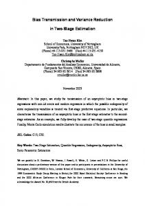
A benchmark resonant-tunneling diode (RTD) has been chosen from the literature [7] for simulation experiments. Simulation results obtained by the two MC algoritms and by NEMO–1D based on non-equilibrium Green’s functions [6] are compared. A common physical model is used for all simulations. The effective mass is uniform 0.067 and the barrier height is 0.27eV. The barriers have a thickness of 2.825nm and the well has a thickness of 4.52nm. The doping level in the contacts is 2 · 1018 cm−3 , linear potential drop across the central device is assumed. Fig. (1) compares the current-voltage characteristis of the RTD obtained by the three approaches. A typical (for stochastic methods) variance of the simulation results is demonstrated for moderate simulation times. Convergence is achieved after a very long simulation presented for QMC-II algorithm. The agreement with the deterministic curve

467

Operator-Split Method for Variance Reduction in Stochastic Solutions

7

Electron Concentration (a.u.)

Current Density (10^5A/cm^2)

10

NEMO QMC-II long QMC-II QMC-I

6 5 4 3 2

0.13V, QMC-I 0.13V, QMC-II 0.21V, QMC-I 0.21V, QMC-II barrier

1

0.1

1 0 0

0.05

0.1

0.15 Voltage (V)

0.2

0.25

Figure 1: Current-Voltage characteristics obtained by simulations with NEMO–1D, QMC-I and QMC-II.

0.01 -20

-15

-10

-5

0 x (nm)

5

10

15

20

Figure 2: Comparison of the electron concentrations obtained by simulations with QMC-I and QMC-II.

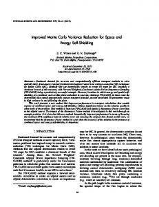
of NEMO–1D solver is good already for the results obtained with moderate simulation times. Fig. (2) shows the electron concentration in the central part of the simulated device as obtained by the two MC algorithms. The chosen voltage values correspond to the peak and valley points of the current-voltage characteristic. The corresponding results are in excellent agreement.

5

Conclusions

The proposed Monte Carlo method has been successfully applied for realistic nanoelectronic devices. Variance reduction has been achieved by annihilation of positive and negative particles into the phase space cells. The particle picture associated to the stochastic process has been used to interpret and explain quantum transport phenomena in Wigner representation.

References [1] W. Frensley, “Boundary conditions for open quantum systems driven far from equilibrium,” Reviews of Modern Physics, vol. 62, no. 3, pp. 745–789, 1990. [2] H. Kosina, M. Nedjalkov, and S. Selberherr, “The Stationary Monte Carlo Method for Device Simulation - Part I: Theory,” J.Appl.Phys., vol. 93, no. 6, pp. 3553–3563, 2003. [3] M. Nedjalkov, H. Kosina, and S. Selberherr, “Monte Carlo Algorithms for Stationary Device Simulation,” Mathematics and Computers in Simulation, vol. 62, no. 3-6, pp. 453–461, 2003. [4] M. Nedjalkov, H. Kosina, and S. Selberherr, “Stochastic Interpretation of the Wigner Transport in Nanostructures,” Microelectronics Journal, vol. 34, pp. 443–445, 2003.

468

M. Nedjalkov, E. Atanassov, H. Kosina and S. Selberherr

[5] C. Wordelman, T. Kwan, and C. Snell, “Comparison of Statistical Enhancement Methods for Monte Carlo Semiconductor Simulation,” IEEE Trans.Computer-Aided Design, vol. 17, no. 12, pp. 1230–1235, 1998. [6] H. Kosina, G. Klimeck, M. Nedjalkov, and S. Selberherr, “Comparison of Numerical Quantum Device Models,” in Proc. Simulation of Semiconductor Processes and Devices, (Boston, USA), pp. 171–174, Sept. 2003. [7] H. Tsuchiya, M. Ogawa, and T. Miyoshi, “Simulation of Quantum Transport in Quantum Devices with Spatially Varying Effective Mass,” IEEE Trans.Electron Devices, vol. 38, no. 6, pp. 1246–1252, 1991.