Optical Flow Estimation using Genetic Algorithms - Semantic Scholar

Optical Flow Estimation using Genetic Algorithms Marco Tagliasacchi1 Politecnico di Milano, Dipartimento di Elettronica e Informazione, Piazza Leonardo da Vinci, 32 20133 Milano, Italy [email protected]

Abstract. This paper illustrates a new optical flow estimation technique, which builds upon a genetic algorithm (GA). First, the current frame is segmented into generic shape regions, using only brightness information. For each region a two-parameter motion model is estimated using a GA. The fittest individuals identified at the end of this step are used to initialise the population of the second step of the algorithm, which estimates a six-parameter affine motion model, again using a GA. The proposed method is compared against a multiresolution version of the well-known Lukas-Kanade differential algorithm. It proved to yield the same or better results in term of energy of the residual error, yet providing a compact representation of the optical flow, making it particularly suitable to video coding applications.

1

Introduction

We refer to the optical flow as the movement of intensity patterns in the 2D space across adjacent frames of an image sequence. Usually, optical flow is the result of the projection on the 2D image plane of the true 3D motion of the objects composing the scene. Optical flow estimation tries to assign to each pixel of the current frame a two-component velocity vector indicating the position of the same pixel in the reference frame. The knowledge of the optical flow is valuable information in several applications, ranging from video coding, motionsegmentation and video surveillance just to name a few. For the rest of this paper, our main scope will be video coding. It should pointed out that a sensible optical flow might be registered also when objects do not move, due to noise, reflections or illumination changes. In this paper we do not try to track real world moving objects, but simply to provide a motion field which minimizes the energy of prediction residuals, after motion compensation. In literature there exists several methods that attempt to estimate optical flow. [1] contains a complete survey comparing most of them. Following the classification proposed in [1], we might arrange them in the following categories: differential (Lukas-Kanade [2], Horn-Schunk [3], Nagel [4]), region-based matching (Anandan [5]), energy-based (Heeger [6]) and phase correlation algorithms (Fleet-Jepson [7]). We chose the

Lukas-Kanade algorithm as a benchmark because it is one of the most performing according to [1]. Moreover it provides a full coverage of the video frame, at least when implemented in a multiresolution fashion, as explained in greater detail in Section 3. Although our algorithm does not match exactly any of the aforementioned categories, it shares similarities with region-based matching methods. In fact both try to find those velocity vectors that maximize the correlation between a pair of consecutive frames; the substantial differences being that our approach substitutes a full search with a genetic algorithm driven search and square blocks with generic shape regions. The remainder of this paper is organized as follows: Section 2 clarifies the metrics that can be used to assess the quality of the estimate. Section 3 summarizes the Lukas-Kanade differential algorithm. Section 4 details the genetic algorithm we employed to perform optical flow estimation. Section 5 is dedicated to experimental results. The paper concludes in Section 6.

2

Metrics to assess estimation

In order to assess the quality of an estimate we can use one of the following two metrics: either the average angular deviation [1] or the energy of the displaced frame difference. The former can be applied only when we are working on synthetic sequences and the real optical flow is know in advance. The deviation is not computed as the simple Euclidean distance between two velocity vectors va = (vax , vay ) and vb = (vbx , vby ). Both are first converted to three component vectors having unitary norm, applying the following transformation: µ ¶ vx vy 1 ve = , , (1) kvk kvk kvk Then, the angular displacement between the two transformed vectors turns out to be: Ψe = arccos hvae , vbe i

(2)

The displaced frame difference (DFD) is computed as the difference between the pixel intensities of the current and the reference frame, following the motion trajectories identified by the optical flow. Stated formally: DF D(xi , yi ) = I (xi , yi , t) − I (xi − vix , y − viy , t − 1)

(3)

In order to assess the estimate we can either compute the energy of the DFD (MSE - mean square error) or the MAD (mean absolute differences). The lower is the MSE or MAD, the better the estimate. It is worth pointing out that, despite average angular deviation, DFD can be applied as a metrics even if the real optical flow is not known, as it is the case for natural imagery. Furthermore, it is more suitable when we are interested in video coding, since our ultimate goal is to reduce the energy of the prediction residuals.

3

Lukas-Kanade differential algorithm

Lukas-Kanade estimation algorithm is one of simplest, yet powerful methods to compute optical flow. For this reason it is one of the most widely used. It builds upon the assumption that the image intensity remains unchanged along motion trajectories: dI(x, y, t) = o(t2 ) dt

(4)

If we add to this equation the brightness smoothness constraint, i.e. that the brightness variation is linear if we look at an about of the location of interest, we obtain: Ix (x, y)vx + Iy (x, y)vy + It (x, y) = 0 (5) Where Ix , Iy and It respectively the horizontal, vertical and temporal gradients. In order to enforce such a constraint, the sequence is pre-filtered along time and space with a gaussian kernel. Equation (5) represents a line in the velocity space. To find a unique solution we impose that the equation might be satisfied for all pixels falling in a window centered on the current pixel, yielding the following over-determined system (6), whose solution is computed using least squares (8):     Ix1 Iy1 · ¸ −It1  Ix2 Iy2  vx  −It2      (6)  ... ...  vy =  ...  IxM IxM −ItM Av = b

(7)

v = (AT A)−1 AT b

(8)

Lukas-Kanade algorithm suffers from the so-called aperture problem, thus it is unable to produce an accurate result when there is not enough texture within the observation window. In this situation it is able to estimate only the component that is parallel to the local gradient. The minimum eigenvalue of the matrix AT A is usually employed as a good indicator. Only when it is greater than a given threshold (approx. 1), a full velocity estimate can be accurately computed. Another drawback of this solution is that it fails to estimate large displacements because the brightness cannot be assumed to be linear far from the observation point. In order to overcome this limitation we can apply a multiresolution approach. A low-pass laplacian pyramid is built and the Lukas-Kanade algorithm runs on the lowest resolution copy. The estimated optical flow is then interpolated and refined at the next level.

4

GA-based optical flow estimation algorithm

The proposed algorithm starts by creating a complete segmentation of the current frame, grouping together those pixels sharing the same spatial location and having similar brightness. We accomplished this task performing a watershed algorithm on a morphological gradient, as explained in [10]. Nevertheless, the segmentation method does not affect the optical flow estimation, thus it will not be described further in this paper. It must be pointed out that there is no connection between the segmentation taking place in successive frames. Our goal is not to describe the temporal evolution of these regions, hence identifying the individual moving objects, rather to produce a dense optical field. We assume that motion field is smooth apart from abrupt changes along object boundaries. Therefore each region is a moving object (or, more likely, part of a larger moving object) and its pixels have a coherent motion that can be described with a limited number of parameters. In this paper we suppose a six-parameter affine motion model. An affine model is able to capture the motion of a rigid planar surface, which moves on the 3D space, projected on the 2D image plane. Although real objects are not planar indeed, this is a good approximation, since it allows describing complex motion such as zooming, rotation and shear. Once the six motion parameters are known, the full velocity vectors at any point (x,y) of the current region can be computed as: xi yi + a5 Cx Cy xi yi = a2 + a4 + a6 Cx Cy

vix = a1 + a3 viy

(9)

Where a = (a1, a2, a3, a4, a5, a6, ) is the motion model vector, Cx and Cy the region centroid coordinates. Having fixed the motion model, it is matter of finding the vector a which minimize the MSE: M

a = arg min

1 X |I(xi , yi , t) − I(xi − vix , yi − viy , t − 1)|2 M i=1

(10)

Where M is the number of pixels in the current region. This is an unconstrained non-linear optimization problem in a six-variable space, characterized by the following features: the function to be minimized should not be expressed in an explicit form the search space is large there are several local optima a good solution, even if it is not the global optimum, might be satisfactory Although conventional multivariate optimization algorithm might be used, we decided to investigate the adoption of genetic algorithms in order to find the solution, since they are well suited to this class of problems.

In order to speed up the convergence, the algorithm is divided into two phases. Step I computes the estimate of a simpler two-parameter model, which is able to describe only rigid translations. The result is used to initialise Step II, which refines the solution estimating the whole six-parameter affine model. Only the fittest half of the population is selected at the end of Step I, and it is mixed with a randomly generated population. The individuals of the genetic algorithm are encoded as 48 bits binary string chromosome, where each variable is represented with a precision of 8 bits. This allows to span the interval [-16,+16] with 1/8 pixel accuracy. The initial population is selected at random, dragging samples from a gaussian distribution. The objective function is used to provide a measure of how individuals have performed in the problem domain. In the case of a minimization problem, the fittest individuals will have the lowest numerical value of the associated objective function. In our problem scope, the objective function is the energy of the DFD, computed for a given vector a = (a1, a2, a3, a4, a5, a6, ): M

f (x) =

1 X 2 |I(xi , yi , t) − I(xi − vix , yi − viy , t − 1)| = M i=1

(11)

M

1 X |I(xi , yi , t)+ M i=1 xi yi xi yi + a5 ), yi − (a2 + a4 + a6 ), t − 1) − I(xi − (a1 + a3 Cx Cy Cx Cy =

(12)

We make the assumption that the magnitude of vx and vy cannot be larger than 20 pixels. In this case the computation of the objective function is stopped prematurely, in order to speed up the evaluation. The fitness of an individual is calculated from the objective function using linear ranking, with selective pressure equal to 2. F (pi ) = 2

pi − 1 Nind − 1

(13)

Where pi is the position in the ordered population of individual i, using the value of the objective function as a ranking criterion. Nind is the number of individuals in the current population, which has been set to 20 in our experiments. The selection phase extracts the individuals that have to be reproduced using stochastic universal sampling, which guarantees zero bias and minimum spread. A generation gap of 0.9 is chosen in order to maintain the fittest individuals. Multipoint crossover is performed on pairs of chromosomes with probability 0.7. The crossover points have fixed locations, corresponding to the boundaries between the variables, in order to preserve the building blocks. Mutation probability is set to 0.7/Lind , where Lind is the length of the chromosome. This value is selected as it implies that the probability of any one element of a chromosome being mutated is approximately 0.5 [9]. Each step of the algorithm is teminated when the objective function computed for the fittest individual has not changed

during the last 10 iterations. Both Step I and Step II use the same design parameters. Experiments demonstrate that with this configuration, the algorithm converges in less than 40 generations, 20 of which always spent to validate the solution. Figure 3 shows an example that illustrates the convergence. Most of the complexity load is owed to the computation of the objective function, which grows linearly with the area of the regions. However, once the segmentation of the current frame is performed, the algorithm works independently on each region. This observation suggests that it suits a parallel implementation, where the number of simultaneous tasks matches the number of regions. Therefore, the time complexity turns out to be of the order O(LN M/K), where L is the average number of iteration for the genetic algorithm to converge, N and M respectively the frame height and width, while K is the number of regions. Our algorithm does not require demanding memory requirements, since only two frame buffers are used at a time to store the current and the reference frame. With respect to Lukas-Kanade, which requires two parameters for each pixel to be represented, our algorithm provides a more compact representation, since it uses only six parameters for each region. Despite of this, experimental results demonstrate that the accuracy of the estimate is not affected, since the affine model seems to capture adequately the motion of most natural scenes. Moreover, the algorithm does not impose the brightness smoothness constraint and it is supposed to work well even in case of poor local texturing. For this reason it always guarantees complete coverage.

5

Experimental results

In this section we compare the results we have obtained with our algorithm (GA) with the ones of Lukas-Kanade, in its multiresolution version (LK1) as discussed in Section 3. Moreover, in order to make a fair comparison, we computed an a posteriori compact representation of the Lukas-Kanade optical flow, estimating by weighted least squares the affine motion model that best fits the data in each segmented region. In order to improve the estimate of the affine model, each pixel is assigned a weight reflecting its reliability. Pixels located close to the border and those having a non-textured neighbourhood receive a lower weight. Segmentation and optical flow estimation are performed independently and they are merged only at last. We will refer to this variant as LK2. We performed our tests on the synthetically generated Yosemite sequence (see Figure 1). Since the real optical flow is available, we are able to compute both the MSE of the DFD and the angular deviation, which are listed in Table 1. The tabulated value of the angular deviation for LK1 differs from the one reported in literature ([1]) for two reasons: a) the latter refers to a coverage of only 40% obtained with a single resolution approach; b) a 15 pixel wide border, i.e. where most of the error is concentrated, is not considered. GA and LK1 outperform LK2 in terms of MSE. With respect to the average angular deviation, GA performs better than LK1. A closer inspection demonstrates that this is especially true along image borders. LK2 perform significantly better

using this metrics. The reason is that the regularization performed by the affine model filters out outliers, improving the estimate at a cost of higher MSE. These results are confirmed by those obtained for the Foreman sequence (see Figure 2). In this case, GA reaches a MSE lower than LK1, while LK2 performs slightly worse.

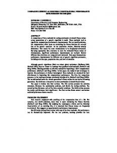
Fig. 1. Estimated optical flow of the Fig. 2. Estimated optical flow of the ForeYosemite sequence, frame 10 man sequence, frame 193

Table 1. Yosemite

Table 2. Foreman

Avg. Ang. Dev. MSE GA 12.1288 50.3302 LK1 14.0553 50.2521 LK2 9.7363 54.1814

MSE GA 25.9856 LK1 29.2421 LK2 34.6167

We did another experiment aimed at determining the optimal stopping criterion. We stated that both Step I and Step II stop when the best individual objective function has not changed during the last G generations. Figure 4 shows the relation existing between G and the quality of the estimate for the Foreman sequence. By increasing G the average number of generations for each region and the time needed to complete the algorithm grow. For this reason, setting G equal to 10 is a good trade-off between quality and complexity.

6

Conclusions

In this paper we introduced a new optical flow estimation method that takes advantage of a two-step genetic algorithm. Experiments proved that it yields results comparable to the Lukas-Kanade algorithm, yet providing a compact representation of the optical flow, suitable for coding applications. We are currently working on a multiresolution version of the algorithm aiming at speeding up the computation. The presented method will be used as the core component

Fig. 3. Sample generations. Objective Fig. 4. Effect of the stopping criterion G function value of the fittest individual. on the MSE and time complexity Red: Step I, blue: Step II

of a motion segmentation algorithm whose goal is to isolate distinct moving objects composing the scene.

References [1] J.L. Barron, D.J. Fleet, and S.S. Beauchemin, “Performance of Optical Flow Techniques”. In International Journal of Computer Vision, February 1994, vol. 12(1), pp. 43—77. [2] B. Lucas and T. Kanade. “An iterative image registration technique with an application to stereo vision”. In Proceedings of the International Joint Conference on Artificial Intelligence, 1981. [3] B.K.P. Horn, B.G. Schunk. “Determining optical flow”. In AI 17, pp. 185-204, 1981 [4] H.H. Nagel. “On the estimation of optical flow: Relations between different approaches and somenew results”. In AI 33, pp.299-324, 1987 [5] P. Anandan. “A computational framework and an algorithm for the measurement of visual motion”. In Int. J. Comp. Vision 2, pp.283-310, 1989 [6] D.J. Heeger, “Optical flow using spatiotemporal filters”. In Int. J. Comp. Vision 1, pp.279-302, 1988 [7] D.J. Fleet, A.D. Jepson. “Computation of component image velocity from local phase information”. In Int. J. Comp. Vision 5, pp.77-104, 1990 [8] J.R. Bergen, P. Anandan, K.J. Hanna, and R. Hingorani. “Hierarchical modelbased motion estimation”. In Proceedings of the European Conference on Computer Vision, 1992. [9] L. Booker, “Improving search in genetic algorithms”. In Genetic Algorithms and Simulated Annealing, L. Davis (Ed.), pp. 61-73, Morgan Kaufmann Publishers, 1987. [10] D. Wang, “A multiscale gradient algorithm for image segmentation using watersheds”. In Pattern Recognition, vol. 678, no. 12, pp. 2043-2052, 1997