Optimal broadcast domination of arbitrary graphs in polynomial time? Pinar Heggernes and Daniel Lokshtanov Department of Informatics, University of Bergen, N-5020 Bergen, Norway.
[email protected],
[email protected]
Abstract. Broadcast domination was introduced by Erwin in 2002, and it is a variant of the standard dominating set problem, such that vertices can be assigned various domination powers. Broadcast domination assigns a power f (v) ≥ 0 to each vertex v of a given graph, such that every vertex of the graph is within distance f (v) from some vertex v having f (v) ≥ 1. The optimal broadcast domination problem seeks to minimize the sum of the powers assigned to the vertices of the graph. Since the presentation of this problem its computational complexity has been open, and the general belief has been that it might be N P-hard. In this paper, we show that optimal broadcast domination is actually in P, and we give a polynomial time algorithm for solving the problem on arbitrary graphs, using a non standard approach.
1
Introduction
A dominating set in a graph is a subset of the vertices of the graph such that every vertex of the graph either belongs to the dominating set or has a neighbor in the dominating set. A vertex outside of the dominating set is said to be dominated by one of its neighbors in the dominating set. The standard optimal domination problem seeks to find a dominating set of minimum cardinality. Since the introduction of this problem [2], [12], many domination related graph parameters have been introduced and studied, and domination in graphs is one of the most well known and widely studied subjects within graph algorithms [7], [8]. The standard dominating set problem can be seen as to represent a set of cities having broadcast stations, where every city can hear a broadcast station placed in it or in a neighboring city [11]. In 2002 Erwin [5] introduced the broadcast domination problem, which is more realistic in the sense that the various broadcast stations are allowed to transmit at different powers. FM radio stations are distinguished both by their transmission frequency and by their ERP (Effective Radiated Power). A transmitter with a higher ERP can transmit further, but it is more expensive to build and to operate. Consequently, the optimal broadcast domination problem asks to compute an integer valued power function ?
This work is supported by the Research Council of Norway through the SPECTRUM project grant.
f on the vertices, such that every vertex of the graph is at distance at most f (v) from some vertex v having f (v) ≥ 1, and the sum of the powers are minimized. Since the introduction of this problem, its computational complexity has been open [4], [10]. The standard optimal domination problem is N P-hard [6], and so are some variants that might resemble broadcast domination: optimal rdomination asks for a dominating set of minimum cardinality where every vertex of the graph is within distance r from some vertex of the dominating set for a given r [9], [13], and the (k, r)-center problem asks to find an r-dominating set containing at most k vertices, where one parameter is given and the other is to be minimized [1], [6]. Since most of the interesting domination problems are N P-hard on general graphs, this gave some indication that optimal broadcast domination might also be N P-hard for general graphs. Following this, in 2003 Blair et al. gave polynomial time algorithms for optimal broadcast domination of trees, interval graphs, and series-parallel graphs [3]. In this paper, we show that, quite surprisingly, optimal broadcast domination is in P. We first prove that every graph has an optimal broadcast domination in which the subsets of vertices dominated by the same vertex are ordered in a path or a cycle. Using this, we give a polynomial time algorithm for computing optimal broadcast dominations of arbitrary graphs. Our algorithm computes minimum weight paths in an auxiliary graph, and thus differs from standard methods of proving polynomial time bounds, like reductions to 2-SAT or 2-dimensional matching. This paper is organized as follows. In the next section, we give the necessary background. In Section 3, we prove the necessary results on the structure of optimal broadcast dominations. In Section 4, we use this result to develop a polynomial time algorithm for all graphs. We conclude with a few remarks in Section 5.
2
Definitions and terminology
In this paper we work with unweighted, undirected, connected, and simple graphs as input graphs to our problem. Let G = (V, E) be a graph with n = |V | and m = |E|. For any vertex v ∈ V , the neighborhood of v is the set NG (v) = {u | uv ∈ E}. Similarly, for any set S ⊆ V , NG (S) = ∪v∈S N (v) − S. We let G(S) denote the subgraph of G induced by S. The distance between two vertices u and v in G, denoted by dG (u, v), is the minimum number of edges on a path between u and v. The eccentricity of a vertex v, denoted by e(v), is the largest distance from v to to any vertex of G. The radius of G, denoted by rad(G), is smallest eccentricity in G. The diameter of G, denoted by diam(G), is the largest distance between any pair of vertices in G. A function f : V → {0, 1, · · · , diam(G)} is a broadcast on G. The set of broadcast dominators defined by f is the set Vf = {v ∈ V | f (v) ≥ 1}. A broadcast is dominating if for every vertex u ∈ V there is a vertex v ∈ Vf such that d(u, v) ≤ f (v). In this case f is also called a broadcast domination. The cost
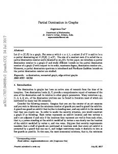
P of a broadcast f incurred by a set S ⊆ V is cf (S) = v∈S f (v). Thus, cf (V ) is the total cost incurred by broadcast function f on G. For a vertex v ∈ V and an integer p ≥ 1, we define the ball BG (v, p) to be the set of vertices that are at distance ≤ p from v in G. Thus BG (v, f (v)) is the set of all vertices that are dominated by v (including v itself) if f (v) ≥ 1. We will omit the subscript G in the notation for balls, since a ball will always refer to the input graph G. A broadcast domination f on G is efficient if B(u, f (u))∩B(v, f (v)) = ∅ for all pairs of distinct vertices u, v ∈ V . For an efficient broadcast domination f on G, we define the domination graph Gf = (Vf , {uv | NG (B(u, f (u)))∩B(v, f (v)) 6= ∅}). Hence the domination graph can be seen as a modification of G in which every ball B(v, f (v)) is contracted to the single vertex v, and neighborhoods are preserved. Since G is connected and f is dominating, Gf is always connected. An example is given in Figure 1.
(1)
(1)
x
y (1)
z
x
(1)
z
(2)
y
(2)
Fig. 1. On the left hand side, a graph G with an efficient broadcast domination f is shown. For vertices v with f (v) ≥ 1, the broadcast powers f (v) are shown in parentheses, and the dashed curves indicate the balls B(v, f (v)). For all other vertices w, f (w) = 0. On the right hand side, the corresponding domination graph Gf is given, and the weight of each vertex is shown in parentheses.
The optimal broadcast domination problem on a given graph G asks to compute a broadcast domination on G with the minimum cost. Note that if f is an optimal broadcast domination on G = (V, E), then cf (V ) ≤ rad(G) since one can always choose a vertex v of smallest eccentricity and dominate all other vertices with f (v) = e(v) = rad(G). If cf (V ) = rad(G) = f (v) for a single vertex v in G, then f is called a radial broadcast domination.
3
The structure of an optimal broadcast domination
In [4], Dunbar et al. show that every graph has an optimal broadcast domination that is efficient. In particular, the following lemma is implicit from the proof of this result. Lemma 1. (Dunbar et al. [4]) For any non efficient broadcast domination f on a graph G = (V, E), there is an efficient broadcast domination f 0 on G such that |Vf 0 | < |Vf | and cf 0 (V ) = cf (V ). We now add the following results. Lemma 2. Let f be an efficient broadcast domination on G = (V, E). If the domination graph Gf has a vertex of degree > 2, then there is an efficient broadcast domination f 0 on G such that |Vf 0 | < |Vf | and cf 0 (V ) = cf (V ). Proof. Let v be a vertex with degree > 2 in Gf , and let x, y, and z be three of the neighbors of v in Gf . By the way the domination graph Gf is defined, v, x, y, and z are also vertices in G, and they all have broadcast powers ≥ 1 in f . Since f is efficient, dG (v, x) = f (v) + f (x) + 1. Similarly, dG (v, y) = f (v) + f (y) + 1 and dG (v, z) = f (v) + f (z) + 1. Assume without loss of generality that f (x) ≤ f (y) ≤ f (z). If f (x) + f (y) > f (z) then we construct a new broadcast f 0 on G with 0 f (u) = f (u) for all vertices u ∈ V \ {v, x, y, z}. Furthermore, we let f 0 (v) = f (v) + f (x) + f (y) + f (z), and f 0 (x) = f 0 (y) = f 0 (z) = 0. The new broadcast f 0 is dominating since every vertex that was previously dominated by one of v, x, y, or z is now dominated by v. To see this, let u be any vertex that was dominated by x, y, or z in f . Thus dG (v, u) ≤ f (v) + 2f (z) + 1 by our assumptions. Since f 0 (v) > f (v) + 2f (z), vertex u is now dominated by v in f 0 . The cost of f 0 is the same as that of f , and the number of broadcast dominators in f 0 is smaller. Let now f (x) + f (y) ≤ f (z). As we mentioned above, there is a path P in G between v and z of length f (v) + f (z) + 1. Let w be a vertex on P such that the number of edges between w and z on P is f (v) + f (x) + f (y). Since f is efficient, f (w) = 0. We construct a new broadcast f 0 on G such that f 0 (u) = f (u) for all vertices u ∈ V \ {v, w, x, y, z}. Furthermore, we let f 0 (w) = f (v) + f (x) + f (y) + f (z), and f 0 (v) = f 0 (x) = f 0 (y) = f 0 (z) = 0. By the way dG (z, w) is defined, any vertex that was dominated by z or v in f is now dominated by w, since dG (v, w) < f (z). Let u be a vertex that was dominated by y in f . The distance between u and w in G is ≤ 2f (y) + 2f (v) + f (z) + 2 − f (v) − f (x) − f (y) = f (y) + f (v) + f (z) + 2 − f (x) ≤ f (y) + f (v) + f (z) + f (x) = f 0 (w). Thus u is now dominated by w. The same is true for any vertex that was dominated by x in f since we assumed that f (x) ≤ f (y). Thus f 0 is a broadcast domination. Clearly, the costs of f 0 and f are the same, and f 0 has fewer broadcast dominators. Thus we have shown how to compute a new broadcast domination f 0 as desired. If f 0 is not efficient, then by Lemma 1 there exists an efficient broadcast domination with the same cost and fewer broadcast dominators, so the lemma follows.
We are now ready to state the main result of this section, on which our algorithm will be based. Theorem 1. For any graph G, there is an efficient optimal broadcast domination f on G such that the domination graph Gf is either a path or a cycle. Proof. Let f be any efficient optimal broadcast domination on G = (V, E). If Gf has a vertex of degree > 2 then by Lemma 2, an efficient broadcast domination f 0 on G with |Vf 0 | < |Vf | and cf 0 (V ) = cf (V ) exists. The proofs of both Lemmas 1 and 2 are constructive, so we know how to obtain f 0 . As long as there are vertices of degree > 2 in the domination graph, this process can be repeated. Since we always obtain a new domination graph with a strictly smaller number of vertices, the process has to stop after < n steps. Since domination graphs are connected, the theorem follows. Note that a path can be a single edge or a single vertex. If Gf is a single vertex then f is a radial broadcast. Corollary 1. For any graph G = (V, E), there is an efficient optimal broadcast domination f on G such that removing the vertices of B(v, f (v)) from G results in at most two connected components, for every v ∈ Vf . Proof. Since there is always an efficient optimal broadcast domination f on G such that the balls B(v, f (v)) with v ∈ Vf are ordered in a path or a cycle by Theorem 1, it suffices to observe that B(v, f (v)) induces a connected subgraph in G for each v ∈ Vf . Corollary 2. For any graph G = (V, E), there is an efficient optimal broadcast domination f on G such that a vertex x ∈ Vf satisfies the following: G0 = G(V \ B(x, f (x))) is connected (or empty), and G0 has an efficient optimal broadcast domination f 0 such that G0f 0 is a path (or empty). Proof. By Theorem 1, let f be an efficient optimal broadcast domination of G such that Gf is a path or a cycle. Let x be any vertex of Gf if Gf is a cycle, any of the two endpoints of Gf if Gf is a path with at least two vertices, or Gf itself if Gf is a single vertex. Let f 0 (v) = f (v) for all v ∈ V \ {x}. Since f is efficient on G, f 0 is an efficient dominating broadcast on G0 , and G0f 0 is the result of removing x from Gf . Thus G0f 0 is a path or empty.
4
Computing an optimal broadcast domination
By Theorem 1 we know that an efficient optimal broadcast f on G must exist such that Gf is a path or a cycle. We will first give an algorithm for handling the case when Gf is a path.
4.1
Optimal broadcast domination when the domination graph is a path
In this subsection, we want to find an efficient broadcast domination of minimum cost over all broadcast dominations f on G = (V, E) such that Gf is a path. Our approach will be as follows: for each vertex u of G, we will compute a new graph Gu , and use this to find the best possible broadcast domination f such that Gf is a path and u belongs to a ball corresponding to one of the endpoints of Gf . We will repeat this process for every u in G, and choose at the end the best f ever computed. Given a vertex u ∈ V , we define a directed graph Gu with weights assigned to its vertices as follows: For each v ∈ V and each p ∈ [1, ..., rad(G)], there is a vertex (v, p) in Gu if and only if one of the following is true: • G(V \ B(v, p)) is connected or empty and u ∈ B(v, p) • G(V \ B(v, p)) has at most two connected components and u 6∈ B(v, p). Thus Gu has a total of at most n · rad(G) vertices. Following Corollaries 1 and 2, each vertex (v, p) represents the situation that f (v) = p in the broadcast domination f that we are aiming to compute. We define the weight of each vertex (v, p) to be p. The role of u is to define the “left” endpoint of the path that we will compute. All edges will go from “left” to “right”. We partition the vertex set of Gu into four subsets: • Au = {(v, p) | G(V \ B(v, p)) is connected and u ∈ B(v, p)} • Bu = {(v, p) | G(V \ B(v, p)) has two connected components} • Cu = {(v, p) | G(V \ B(v, p)) is connected and u 6∈ B(v, p)} • Du = {(v, p) | B(v, p) = V } For each vertex (v, p), let Lu (v, p) be the connected component of G(V \ B(v, p)) that contains u (i.e., the component to the “left” of B(v, p)), and let Ru (v, p) be the connected component of G(V \ B(v, p)) that does not contain u (i.e., the component to the “right” of B(v, p)). Thus Lu (v, p) = ∅ for every (v, p) ∈ Au ∪ Du , and Ru (v, p) = ∅ for every (v, p) ∈ Cu ∪ Du . The edges of Gu are directed and defined as follows: A directed edge (v, p) → (w, q) is an edge of Gu if and only if all of the following three conditions are satisfied: • B(v, p) ∩ B(w, q) = ∅ in G • Ru (v, p) 6= ∅ and Lu (w, q) 6= ∅ • (NG (B(w, q)) ∩ Lu (w, q)) ⊂ B(v, p) and (NG (B(v, p)) ∩ Ru (v, p)) ⊂ B(w, q) in G. To restate the last requirement in plain text: B(v, p) must contain all neighbors of B(w, q) in Lu (w, q), and B(w, q) must contain all neighbors of B(v, p) in Ru (v, p). Observation 1 Given the first two requirements that an edge of Gu must satisfy, the two conditions of the last requirement are equivalent. Proof. Note first that (NG (B(w, q)) ∩ Lu (w, q)) 6= B(v, p) and (NG (B(v, p)) ∩ Ru (v, p)) 6= B(w, q) since B(v, p) ∩ B(w, q) = ∅ and thus v has no neighbor
in B(w, q) and w has no neighbor in B(v, p) in G. Let now (NG (B(w, q)) ∩ Lu (w, q)) ⊂ B(v, p). Observe that B(v, p) ⊆ Lu (w, q), since B(v, p)∩B(w, q) = ∅ and each ball induces a connected subgraph of G. Furthermore, since B(w, q) ∪ Ru (w, q) is connected and does not intersect with B(v, p), and since there is no path from B(w, q) to u that avoids B(v, p), we can also conclude that B(w, q) ⊆ Ru (v, p). Assume now, for a contradiction, that (NG (B(v, p)) ∩ Ru (v, p)) 6⊂ B(w, q). Thus B(v, p) has a neighbor z in Ru (v, p) and z 6∈ B(w, q). Since Ru (v, p) is connected there is a path between z and a vertex of B(w, q) in Ru (v, p), and in particular, this path contains a vertex y of Ru (w, q). But this means that there is a path between u and y in G(V \ B(w, q)), which contradicts that y ∈ Ru (w, q). The proof in the other direction is analogous. By the way we have defined the edges of Gu , all vertices belonging to Au have indegree 0 and all vertices belonging to Cu have outdegree 0. Hence, any path in Gu can contain at most one vertex from Au (which must be the starting point of the path) and at most one vertex from Cu (which must be the ending point of the path). The vertices of Du are isolated, and every vertex of Du defines a radial broadcast domination on its own. Lemma 3. Given G = (V, E) and a vertex u in G, let (v1 , p1 ) → (v2 , p2 ) → ... → (vk , pk ) be a directed path in Gu with (v1 , p1 ) ∈ Au ∪ Du and (vk , pk ) ∈ Si−1 Cu ∪ Du . Then for 1 ≤ i ≤ k, the following is true: j=1 B(vj , pj ) = Lu (vi , pi ) Sk and j=i+1 B(vj , pj ) = Ru (vi , pi ). Proof. Observe that k = 1 if and only if the path contains a vertex of Du , in which case the lemma follows trivially. Let us for the rest of the proof assume that k ≥ 2. Si−1 We first show that j=1 B(vj , pj ) = Lu (vi , pi ) by induction on i, starting from i = 1 and continuing to i = k. Let us consider the base cases i = 1 and i = 2. When i = 1, we must show that Lu (v1 , p1 ) = ∅, which follows trivially since (v1 , p1 ) ∈ Au ∪ Du . When i = 2, we need to show that B(v1 , p1 ) = Lu (v2 , p2 ). Since (v1 , p1 ) → (v2 , p2 ) is an edge of Gu and Lu (v1 , p1 ) = ∅, we know that NG (B(v1 , p1 )) ⊂ B(v2 , p2 ). By the definition of an edge of Gu , we also know that NG (B(v2 , p2 )) ∩ Lu (v2 , p2 ) ⊂ B(v1 , p1 ). Thus there cannot exist a path between a vertex of B(v2 , p2 ) and a vertex of B(v1 , p1 ) that avoids B(v1 , p1 ) and the result follows since Lu (v2 , p2 ) is connected. Si−1 For the induction step, assume that j=1 B(vj , pj ) = Lu (vi , pi ), and we Si will show that j=1 B(vj , pj ) = Lu (vi+1 , pi+1 ). Because of the edge (vi , pi ) → (vi+1 , pi+1 ), by the proof of Observation 1, we know that B(vi , pi ) ⊆ Lu (vi+1 , pi+1 ) and B(vi+1 , pi+1 ) ⊆ Ru (vi , pi ). Thus, by the induction assumption, B(vi+1 , pi+1 ) Si does not intersect with j=1 B(vj , pj ). Again by the induction assumption, Si j=1 B(vj , pj ) is connected and contains u. As a consequence, we can conclude Si that j=1 B(vj , pj ) ⊆ Lu (vi+1 , pi+1 ). Now, if Lu (vi+1 , pi+1 ) contains a vertex x S that does not belong to ij=1 B(vj , pj ) then due to the induction assumption,
there must be a path (possibly a single edge) between x and a vertex of B(vi , pi ) Si−1 whose vertices are all outside of j=1 B(vj , pj ). Consequently, B(vi , pi ) must have a neighbor y in Ru (vi , pi ) such that that x 6∈ B(vi+1 , pi+1 ), which contraS dicts the existence of the edge (vi , pi ) → (vi+1 , pi+1 ). Thus ij=1 B(vj , pj ) = Lu (vi+1 , pi+1 ), and the proof of this part is complete. Sk Showing that j=i+1 B(vj , pj ) = Ru (vi , pi ) for 1 ≤ i ≤ k is completely analogous, and we skip this part. Lemma 4. Given G = (V, E), there is a vertex u ∈ V such that (v1 , p1 ) → (v2 , p2 ) → ... → (vk , pk ) is a directed path in Gu with (v1 , p1 ) ∈ Au ∪ Du and (vk , pk ) ∈ Cu ∪ Du if and only if G has an efficient broadcast domination f such that Gf is the undirected path v1 − v2 − ... − vk and f (vi ) = pi for 1 ≤ i ≤ k. Proof. Let f be an efficient broadcast on G = (V, E) with broadcast dominators Vf ⊂ V such that Gf is a path. Let Vf = {v1 , v2 , ..., vk } so that v1 − v2 − ... − vk is the path equivalent to Gf , and let u be any vertex of B(v1 , f (v1 )). If k = 1 then V = B(v1 , p1 ), and the lemma trivially follows since Gu contains a vertex (v1 , p1 ) ∈ Du . Let k ≥ 2. By the proofs of Corollaries 1 and 2, removing B(v1 , f (v1 )) or B(vk , f (vk )) from G results in a connected graph, and removing B(vi , f (vi )) from G results in exactly two connected components for 2 ≤ i ≤ k−1 (if k ≥ 3). Consequently, for each vi ∈ Vf , (vi , f (vi )) is a vertex of Gu . In Gu , (v1 , f (v1 )) belongs to Au , (vk , f (vk )) belongs to Cu , vertices (vi , f (vi )) belong to Bu for 2 ≤ i ≤ k−1 (for k ≥ 3), and (v1 , f (v1 )) → (v2 , f (v2 )) → ... → (vk , f (vk )) is a path by the definition of the edges in Gu . In the other direction, let u be a vertex of G, and let P = (v1 , p1 ) → (v2 , p2 ) → ... → (vk , pk ) be a directed path in Gu such that (v1 , p1 ) ∈ Au ∪ Du and (vk , pk ) ∈ Cu ∪ Du . Define a function f so that f (vi ) = pi for 1 ≤ i ≤ k, Sk and f (v) = 0 for all other vertices of G. By Lemma 3, i=1 B(vi , pi ) = V , and B(vi , pi ) ∩ B(vj , pj ) = ∅, for 1 ≤ i < j ≤ k. Thus f is an efficient broadcast domination on G. Now the idea is to find a directed path Pu in Gu from a vertex of Au ∪ Du to a vertex of Cu ∪ Du such that the sum of the weights of the vertices of Pu (including the endpoints) is minimized. Let us call this sum W (Pu ). Then we will compute Gu for each vertex u in G, and repeat this process, and at the end choose a path with the minimum total weight. Our algorithm for the path case is given in Figure 2. Theorem 2. Given a graph G = (V, E), Algorithm MPBD computes an efficient broadcast domination f on G of minimum cost such that Gf is a path. Proof. We compute a minimum weight path in Gu for every u ∈ V , and among all these paths we choose a path P with the lowest W (P ). By Lemma 4, P corresponds to a broadcast domination f of G such that Gf is a path, and by the way each Gu is constructed, W (P ) = cf (V ). Assume that there is a broadcast domination f 0 on G with cf 0 (V ) < cf (V ) such that Gf 0 is a path. Lemma 4 guarantees the existence of a path P 0 in Gv for some vertex v ∈ V such that W (P 0 ) < W (P ), which is a contradiction.
Algorithm Minimum Path Broadcast Domination - MPBD Input: A graph G = (V, E). Output: An efficient broadcast domination function f of minimum cost on G, such that Gf is a path. begin for each vertex v in G do f (v) = 0; Let P be a dummy path with W (P ) = rad(G) + 1; for each vertex u in G do Compute Gu with vertex sets Au , Bu , Cu , and Du ; Find a minimum weight path Pu starting in a vertex of Au ∪ Du and ending in a vertex of Cu ∪ Du ; if W (Pu ) < W (P ) then P = Pu ; end-for for each vertex (v, p) on P do f (v) = p; end Fig. 2. The algorithm for computing the best path broadcast domination.
Corollary 3. Let G = (V, E) be a graph such that there is an efficient optimal broadcast domination on G where the domination graph is a path. Algorithm MPBD computes such a broadcast domination on G. 4.2
Optimal broadcast domination for all cases
Now we want to compute an optimal broadcast domination for any given graph G. Our approach will be as follows. Let x be any vertex of G. For each k between 1 and rad(G) such that G0 = G(V \ B(x, k)) is connected or empty, we run the minimum path broadcast domination algorithm MPBD on G0 . Our algorithm for the general case is given in Figure 3. In this way, we consider all broadcast dominations f whose corresponding domination graphs are paths or cycles. The advantage of this approach is its simplicity. The disadvantage is that we also consider many cases that do not correspond to a path or a cycle, which we could have detected with a longer and more involved algorithm. However, these unnecessary cases do not threaten the correctness of the algorithm, and detecting them does not decrease the asymptotic time bound. Theorem 3. Algorithm OBD computes an optimal broadcast domination of any given graph. Proof. Let G = (V, E) be the input graph. By Theorem 1 and Corollary 2, there is a vertex x in V and an integer k ∈ [1, rad(G)] such that the graph G0 = G(V \ B(x, k)) has an efficient optimal broadcast domination f 0 where the domination
Algorithm Optimal Broadcast Domination - OBD Input: A graph G = (V, E). Output: An efficient optimal broadcast domination function f on G. begin opt = rad(G) + 1; for each vertex x in G do for k = 1 to rad(G) do if G0 = G(V \ B(x, k)) is connected or empty then f = MPBD(G0 ); if cf (V \ B(x, k)) + k < opt then opt = cf (V \ B(x, k)) + k; f (x) = k; for each vertex v in B(x, k) \ {x} do f (v) = 0; end-if end-if end
Fig. 3. The algorithm for computing an optimal broadcast domination.
graph G0f 0 is a path, and that f 0 can be extended to an optimal broadcast domination f for G with f (x) = k, f (v) = 0 for v ∈ B(x, k) with x 6= v, and f (v) = f 0 (v) for all other vertices v. Algorithm MPBD computes an optimal broadcast domination of G0 , and since Algorithm OBD tries all possibilities for (x, k), the result follows. Note that although there is always an efficient optimal broadcast domination f such that Gf is a cycle or a path, there can of course exist other optimal broadcast dominations f 0 with cf 0 (V ) = cf (V ) such that Gf 0 is not a path or a cycle, and such that f 0 is not efficient. The optimal broadcast domination returned by algorithm OBD does not necessarily correspond to a path or a cycle, since we do not force the endpoints (or forbid the interior points) of the path for G0 to be neighbors of B(x, k). Nor is the returned broadcast necessarily efficient, as some ball B(v, p) might have an outreach outside of G0 and might overlap with B(x, k). 4.3
Time complexity
We explain a straight forward implementation of our algorithms to justify the polynomial time complexity. In Algorithm MPBD, given a graph G, for each vertex u in G, we create an auxiliary graph Gu with at most n · rad(G) vertices. Thus we create n graphs with O(n2 ) vertices and O(n4 ) edges each. In each such graph, we first compute vertex sets Au , Bu , Cu , and Du , which requires a breadth first search for each vertex of Gu , thus O(n6 ) time for each auxiliary graph. The edges of Gu can also be computed within this bound. Then we compute a path of minimum weight in each such graph. A shortest path in a connected graph
H = (U, D) can be computed in time O(|D| log |U |) by well-known algorithms like the one by Dijkstra. Minimum weight paths can be computed by simple modifications of such algorithms within the same time bound. Thus in each graph that we create, it takes O(n4 log n) time to find a minimum weight path. Consequently the total time required for each Gu is O(n6 ), giving a total of O(n7 ) time for Algorithm MPBD. In Algorithm OBD, we repeat this process n · rad(G) = O(n2 ) times to find an optimal broadcast domination. As a result, the overall time complexity of a straight forward implementation is O(n9 ) and thus polynomial. It can be shown that each auxiliary graph Gu is acyclic and has O(n3 ) edges. Therefore minimum weight paths can be computed by topological sort in time O(n3 ) in each such graph. With a preprocessing step of computing all pairs of shortest paths on G in O(n3 ) time, and using an O(n3 ) space data structure to store the information about the edges between all possible balls in all auxiliary graphs, we can actually reduce the total running time to O(n3 r2 m), where r = rad(G). We leave the details of this implementation to the full paper, due to limited space here.
5
Concluding remarks
In this paper we have shown that the broadcast domination problem is solvable in polynomial time on all graphs. Our focus has been on polynomial time and not the best possible time bound. Our algorithm can be enhanced to run substantially faster, as explained. For further research, more efficient algorithms for this problem should be of interest. P The optimal broadcast domination problem studies the cost cf (V ) = v∈V f (v) of a broadcast domination f on a graph G = (V, E). Other definitions of the cost of a broadcast may be appropriate depending on the application, since the cost of a broadcast can be different from the value of a broadcast. To be more precise, P one could define a cost function c(i), and let the total cost be cf (V ) = v∈V c(f (v)). Thus in our case c(i) = i for all i. Our polynomial time algorithm can be used for all cost functions c, where c(i) + c(j) ≥ c(i + j) for all integers i and j ≥ 0. For general cost functions the problem becomes N P-hard, because we can let c(0) = 0, c(1) = 1, and c(i) > n for all i > 1, which gives a direct reduction from the standard dominating set problem.
References 1. J. Bar-Ilan, G. Kortsarz, and D. Peleg. How to allocate network centers. J. Algorithms, 15:385–415, 1993. 2. C. Berge. Theory of Graphs and its Applications. Number 2 in Collection Universitaire de Mathematiques. Dunod, Paris, 1958. 3. J. R. S. Blair, P. Heggernes, S. Horton, and F. Manne. Broadcast domination algorithms for interval graphs, series-parallel graphs, and trees. Congressus Numerantium, 169:55 – 77, 2004.
4. J. E. Dunbar, D. J. Erwin, T. W. Haynes, S. M. Hedetniemi, and S. T. Hedetniemi. Broadcasts in graphs. 2002. Submitted. 5. D. J. Erwin. Dominating broadcasts in graphs. Bull. Inst. Comb. Appl., 42:89–105, 2004. 6. M. R. Garey and D. S. Johnson. Computers and Intractability. W. H. Freeman and Co., 1978. 7. T. W. Haynes, S. T. Hedetniemi, and P. J. Slater. Domination in Graphs: Advanced Topics. Marcel Dekker, New York, 1998. 8. T. W. Haynes, S. T. Hedetniemi, and P. J. Slater. Fundamentals of Domination in Graphs. Marcel Dekker, New York, 1998. 9. M. A. Henning. Distance domination in graphs. In T. W. Haynes, S. T. Hedetniemi, and P. J. Slater, editors, Domination in Graphs: Advanced Topics, pages 321–349. Marcel Dekker, New York, 1998. 10. S. B. Horton, C. N. Meneses, A. Mukherjee, and M. E. Ulucakli. A computational study of the broadcast domination problem. Technical Report 2004-45, DIMACS Center for Discrete Mathematics and Theoretical Computer Science, 2004. 11. C. L. Liu. Introduction to Combinatorial Mathematics. McGraw-Hill, New York, 1968. 12. O. Ore. Theory of Graphs. Number 38 in American Mathematical Society Publications. AMS, Providence, 1962. 13. P. J. Slater. R-domination in graphs. J. Assoc. Comput. Mach., 23:446–450, 1976.