Hindawi Publishing Corporation Scientific Programming Volume 2016, Article ID 4180817, 10 pages http://dx.doi.org/10.1155/2016/4180817
Research Article Optimal Control for Bufferbloat Queue Management Using Indirect Method with Parametric Optimization Amr Radwan,1 Hoang-Linh To,1 and Won-Joo Hwang2 1
Department of Information and Communication System, Inje University, Gimhae, Gyeongnam 50834, Republic of Korea Department of Information and Communications Engineering, HSV-TRC, Inje University, Gimhae, Gyeongnam 50834, Republic of Korea
2
Correspondence should be addressed to Won-Joo Hwang;
[email protected] Received 20 May 2016; Accepted 31 July 2016 Academic Editor: Junhu Ruan Copyright © 2016 Amr Radwan et al. This is an open access article distributed under the Creative Commons Attribution License, which permits unrestricted use, distribution, and reproduction in any medium, provided the original work is properly cited. Because memory buffers become larger and cheaper, they have been put into network devices to reduce the number of loss packets and improve network performance. However, the consequences of large buffers are long queues at network bottlenecks and throughput saturation, which has been recently noticed in research community as bufferbloat phenomenon. To address such issues, in this article, we design a forward-backward optimal control queue algorithm based on an indirect approach with parametric optimization. The cost function which we want to minimize represents a trade-off between queue length and packet loss rate performance. Through the integration of an indirect approach with parametric optimization, our proposal has advantages of scalability and accuracy compared to direct approaches, while still maintaining good throughput and shorter queue length than several existing queue management algorithms. All numerical analysis, simulation in ns-2, and experiment results are provided to solidify the efficiency of our proposal. In detailed comparisons to other conventional algorithms, the proposed procedure can run much faster than direct collocation methods while maintaining a desired short queue (≈40 packets in simulation and 80 (ms) in experiment test).
1. Introduction Nowadays, modern computer networks are incredibly complex and we rely on them to transport huge quantities of data across the globe in seconds. Although this works well, there are some foreseen issues that need to be tackled. As bandwidth-heavy applications such as peer-to-peer networks and websites relying on user-generated content have become more prevalent, especially the relatively slow residential broadband links have been used at full capacity, and interruptions in connectivity have become more common [1]. Recent research has shown that the culprit is the buffers built into network equipment [2]. Accordingly, bufferbloat term has been used to describe related issues whenever these buffers misbehave to produce unnecessary latency [3]. In order to efficiently manage queues which are generated due to the bufferbloat phenomenon, active queue management (AQM) algorithms have been recommended to use in network equipment [4]. Most of the existing
approaches to AQM design exploit feedback control theory with the linearized TCP core model that was proposed by Hollot et al. [5]. The well-known AQMs that monitor the average queue size and drops (or marks) packets based on statistical probabilities are Random Early Detection (RED) [6] or Random Early Marking (REM) [7]. If the buffer is empty, all incoming packets are accepted. When the buffer is full, the probability has reached 1 and all incoming packets are dropped. When queue is growing, the probability grows according to a piecewise linear function and RED (or REM) drops (or marks) packets using the updated probability. The main drawback of RED or REM is that it is sensitive to network parameter changes and requires careful tuning of its parameters in order to provide optimal performance in any scenarios. Recently, in [8], a Proportional Integral Enhanced (PIE) controller as a lightweight AQM is proposed, without the need of per-packet extra processing. Such PItype controllers are known to provide queue control with zero offset (the mean queue length converges to the target value)
2 but are consequently less stable and slower reacting. There have been several other control-theoretic solutions based on feedback fluid-flow model proposed in [9–12] to improve stable and robust control mechanisms, but none of them tackle the issue of system optimality in terms of minimizing both queue length and packet dropping rate performance and searching for an optimal control trajectory. To address such issues, a promising design direction is to reformulate the network queuing problem as an optimal control queue (OCQ) problem [13], where the main state variable is queue length and the control variable is the actual input rate to form the queue [14] or packet dropping rate. Then one of the approaches to solve OCQ is that we can priorly discretize the governing ordinary differential equations (ODEs) and the integral terms in the cost function or constraint functions and thereby replace the infinite dimensional optimal control problem with a large nonlinear optimization problem (NOP). This is known as the direct method in the literature for solving OCQ. This approach is typically easier to use, especially for OCQ with a state equality or inequality constraints. The main difference among direct approaches is how to handle the constraints corresponding to the system dynamics. The three most common direct approaches are direct single shooting, direct multiple shooting, and direct collocation. Direct methods have been used with references in [15–18]. Alternatively, one can first form the optimality conditions, using the calculus of variations and Pontryagin minimum principle, and then solve the resulting boundary value problem. This is known as the indirect method for solving OCQ. The references present just a small sample of the work that discusses or applies indirect methods for the solution of optimal control problems [15, 16, 18, 19]. In rare cases, the solution can be obtained in closed form from the optimality conditions, but, in general, approximation methods are used to solve the problem numerically. The optimality conditions of these problems generally take the form of differential algebraic equations (DAEs) with boundary conditions (BCs). The approximate solution to the OCQ can be obtained by using a boundary value problem (BVP) solver. Perhaps the most popular methods are multiple shooting and collocation. More recently, a combination of direct and indirect methods was proposed leading to hybrid methods [16]. In this paper, we firstly derive methods to solve OCQ using both direct and indirect approaches. We show how to apply the direct collocation approach to solve OCQ problem which can be solved in popular optimization solvers such as JModelica [20] and GAlib [21]. Indirect method with forward-backward for optimal control queue algorithm (FBOCQ) is designed as an alternative to tackle it as well. Our key difference from existing works is that we provide a novel method to update the control step 𝛿𝑢 by solving a parametric optimization subproblem. This method is scalable which means that we can expand for larger problems with more variables as well. The numerical results for both direct and indirect approaches are discussed in Section 5.1 to emphasize our choice of integrating an indirect method with parametric optimization for active queue management design, which is demonstrated more efficiently (i.e., faster reaction and more stable) than direct methods. Finally, we evaluate the proposed
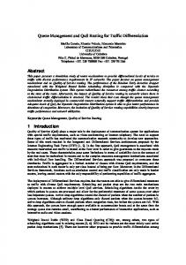
Scientific Programming x(t): queue length u(t): actual rate
w(t): input rate
𝜇 service rate
d(t) = w(t) − u(t): drop rate
Figure 1: OCQ model.
algorithm using network simulator ns-2 and compare it to other AQMs including RED, REM, and PI. The dropping feature of the proposed algorithm makes the average queue length shortened and stabilized compared with others, while throughput is not reduced so much. Our Contributions (i) We present both indirect and direct methods for an optimal control problem which is applied in queue management field (Section 3). The step update 𝛿𝑢 of control variable is calculated by solving a subproblem of parametric optimization with the advantage of scalability. Numerical results show that all of them bring nearly similar results, but indirect method (FBOCQ) is much faster than other solvers and gives the best cost function value (Section 5.1). (ii) We evaluate FB-OCQ in simulation and show that a desired small queue length value at 40 packets can be obtained. Nevertheless, we cannot avoid the tradeoff between queue length and throughput. FB-OCQ’s throughput is slightly smaller than RED’s one (0.075 versus 0.082 Mbps); however, it can be an acceptable value when compared to REM’s and PI’s (Section 5.2). (iii) We implement FB-OCQ in Linux kernel (Ubuntu 16.04) and test it in the worst case using Realtime Response Under Load (RRUL) test suite. The experiment result shows that our algorithm brings low latency ping value compared with the other existing algorithms in Linux kernel (DropTail and RED).
2. Problem Formulation We consider an optimal control model of queue management problem, named (OCQ), in [14] (Figure 1). The main idea is to minimize the cost function which implies a trade-off between queue length and dropping rate, subject to a dynamic constraint of queue length along time 𝑡0 to 𝑡𝑓 as follows: minimize 𝐽 = ∫ 𝑥
subject to
𝑡𝑓
𝑡=0
𝐿 (𝑥 (𝑡) , 𝑢 (𝑡) , 𝑡)
𝑥̇ = 𝑓 (𝑥 (𝑡) , 𝑢 (𝑡) , 𝑡) ,
(OCQ)
0 ≤ 𝑢 (𝑡) ≤ 𝑤 (𝑡) , where 𝐿(𝑥, 𝑢, 𝑡) = 𝑥(𝑡) + 𝑅(𝑤 − 𝑢(𝑡)) is cost function; 𝑓(𝑥(𝑡), 𝑢(𝑡), 𝑡) = 𝑢(𝑡) − 𝜇𝑥/(𝑎 + 𝑥); 𝑅 is weight on dropping rate; 𝑡𝑓 is final time; 𝜇 is service rate (bandwidth capacity); and 𝑎 is parameter for different types of queuing model; for example, when 𝑎 = 1, we obtain an M/M/1 queue.
Scientific Programming
3
3. Numerical Methods for OCQ
and the derivative is
3.1. Direct Method: Collocation Method. In this section, we present how to apply the direct collocation [18] for OCQ. In this method, we discretize the time interval 𝑡0 = 𝑡1 < 𝑡2 < 𝑡3 < ⋅ ⋅ ⋅ < 𝑡𝑘 = 𝑡𝑓 into 𝑁 elements. The state and the total number of packets and control variables at each node are 𝑥𝑗 = 𝑥(𝑡𝑗 ) and 𝑤𝑗 = 𝑤(𝑡𝑗 ) and 𝑢𝑗 = 𝑢(𝑡𝑗 ), such that the state, control, and packets variables at the nodes are defined as nonlinear programming (NLP) variables: 𝑌 = [𝑥 (𝑡1 ) , . . . , 𝑥 (𝑡𝑘 ) , 𝑢 (𝑡1 ) , . . . , 𝑢 (𝑡𝑘 ) , 𝑤 (𝑡1 ) , . . . , 𝑤 (𝑡𝑘 )] .
(1)
The controls are chosen as piecewise linear interpolating functions between 𝑢(𝑡𝑗 ) and 𝑢(𝑡𝑗+1 ) for 𝑡𝑗 ≤ 𝑡 ≤ 𝑡𝑗+1 as follows: 𝑡 − 𝑡𝑗
𝑢app (𝑡) = 𝑢 (𝑡𝑗 ) +
ℎ𝑗
[𝑢 (𝑡𝑗+1 ) − 𝑢 (𝑡𝑗 )] ,
(2)
ℎ𝑗 = 𝑡𝑗+1 − 𝑡𝑗 .
𝑢 (𝑡𝑗 ) + 𝑢 (𝑡𝑗+1 ) 2
,
𝑗 = 1, . . . , 𝑘 − 1.
(3)
The piecewise linear interpolation is used to prepare for the possibility of discontinuous solutions in control. Similarly, we can derive the approximate of the total number of the packets 𝑤app (𝑡) and 𝑤(𝑡𝑗+1/2 ) as above. The state variable 𝑥(𝑡) is approximated by a continuously differentiable and piecewise Hermite-Simpson cubic polynomial between 𝑥(𝑡𝑗 ) and 𝑥(𝑡𝑗+1 ) on the interval 𝑡𝑗 ≤ 𝑡 ≤ 𝑡𝑗+1 of length ℎ𝑗 : 𝑥app (𝑡) =
3
∑𝑐𝑟𝑗 𝑟=0
𝑡 − 𝑡𝑗 ℎ𝑗
3 (𝑥𝑗 + 𝑥𝑗+1 ) 2 (𝑡𝑗+1 + 𝑡𝑗 )
1 (𝑓 + 𝑓𝑗+1 ) , 4 𝑗
(7)
In addition, the chosen interpolating polynomial for the state and control variables must satisfy the midpoint conditions for the differential equations as follows: 𝑓 (𝑥app (𝑡𝑗+1/2 ) , 𝑢app (𝑡𝑗+1/2 ) , 𝑤app (𝑡𝑗+1/2 ) , 𝑡𝑗+1/2 ) − 𝑥̇ app (𝑡𝑗+1/2 ) = 0.
(8)
Equations (OCQ) can now be defined as a discretized problem as follows: min 𝑓 (𝑌)
(9)
𝑓 (𝑥app (𝑡) , 𝑢app (𝑡) , 𝑤app (𝑡) , 𝑡) − 𝑥̇ app = 0,
(10)
𝑥app (𝑡1 ) − 𝑥1 = 0, 0 ≤ 𝑢app (𝑡) ≤ 𝑤app (𝑡) ,
where 𝑥app , 𝑢app , and 𝑤app are the approximations of the state, the control, and the total number of packets, constituting 𝑌 in (9). This above discretization problem (9)-(10) can be solved using the following: (i) JModelica, which is a package for simulation and optimization of Modelica models (for more details see [20]); (ii) GAlib, which is C++ library of genetic algorithm (for more details see [21]).
,
3.2. Indirect Method: Forward-Backward Sweeping. We solve OCQ by using indirect method approach:
𝑗
𝑐0 = 𝑥 (𝑡𝑗 ) , (4)
𝑗
𝑐1 = ℎ𝑗 𝑓𝑗 ,
(i) forming optimality conditions; (ii) solving BVP by First-Order Sweeping algorithm.
𝑗
𝑐2 = −3𝑥 (𝑡𝑗 ) − 2ℎ𝑗 𝑓𝑗 + 3𝑥 (𝑡𝑗+1 ) − (ℎ𝑗 ) 𝑓𝑗+1 ,
Let 𝑥(𝑡) be the adjoint variable. At time 𝑡, let 𝑢∗ (𝑡) denote the optimum controls and let 𝑥∗ (𝑡) and 𝑥∗ (𝑡) denote the state and adjoint evaluated at the optimum. Using Pontryagin minimum principle we get the following equations.
𝑗
𝑐3 = 2𝑥 (𝑡𝑗 ) + ℎ𝑗 𝑓𝑗 − 2𝑥 (𝑡𝑗+1 ) + (ℎ𝑗 ) 𝑓𝑗+1 , where
Hamiltonian Function
𝑓𝑗 = 𝑓 (𝑥 (𝑡𝑗 ) , 𝑢 (𝑡𝑗 ) , 𝑤 (𝑡𝑗 ) , 𝑡𝑗 ) 𝑡𝑗 ≤ 𝑡 ≤ 𝑡𝑗+1 , 𝑗 = 1, . . . , 𝑘 − 1.
(5)
𝐻 (𝑥 (𝑡) , 𝑢 (𝑡) , 𝑥 (𝑡)) = 𝑥 (𝑡) + 𝑅 (𝑤 (𝑡) − 𝑢 (𝑡)) + 𝑥 (𝑡) (𝑢 (𝑡) −
The value of the state variables at the center point 𝑡𝑗+1/2 of the cubic approximation is 𝑥 (𝑡𝑗+1/2 ) =
−
𝑗 = 1, . . . , 𝑘 − 1.
subject to
The value of the control variables at the center 𝑡𝑗+1/2 is given by 𝑢 (𝑡𝑗+1/2 ) =
𝑥̇ (𝑡𝑗+1/2 ) =
𝑥 (𝑡𝑗 ) + 𝑥 (𝑡𝑗+1 ) 2
+
𝑡𝑗+1 + 𝑡𝑗 8
(𝑓𝑗 + 𝑓𝑗+1 ) ,
𝑗 = 1, . . . , 𝑘 − 1,
𝜇𝑥 (𝑡) ). 𝑎 + 𝑥 (𝑡)
(11)
Adjoint Equations (6)
𝑥̇ (𝑡) = −1 + 𝑢 (𝑡)
𝑎𝜇 . (𝑎 + 𝑥 (𝑡))2
(12)
4
Scientific Programming and (𝑢∗ , 𝑥∗ ) satisfies the minimum principle:
Transversality Condition (13)
𝐻 (𝑥∗ , 𝑢∗ , 𝑥∗ ) = min 𝐻 (𝑥∗ , 𝑢, 𝑥∗ ) , 𝑡 ∈ [𝑡0 , 𝑡𝑓 ] . (21) 𝑢∈𝑈
Hamiltonian Minimization Condition. Derivative of the Hamiltonian is evaluated to zero at interior points; hence
(a) First-Order Sweeping Method. We linearize the Hamiltonian around a reference solution 𝑢(𝑡) and obtain the following equation for variation 𝛿𝑢(𝑡):
𝑥 (𝑡𝑓 ) = 0.
𝐻𝑢 (𝑥 (𝑡) , 𝑢 (𝑡) , 𝑥 (𝑡) , 𝜆 (𝑡) , 𝑡) = −𝑅 + 𝑥 (𝑡) − 𝜆 1 (𝑡) + 𝜆 2 (𝑡) = 0.
If 𝑢∗ (𝑡) is optimal in (OCQ), then it must satisfy the minimum condition: 𝐻 (𝑥∗ , 𝑢∗ , 𝑥∗ , 𝑡) = min 𝐻 (𝑥, V, 𝑥, 𝑡) V∈𝑈
∀𝑡 ∈ 𝑁.
(H3) 𝑢 ∈ 𝐶𝑟 [𝑡0 , 𝑡𝑓 ]. Note that 𝑢(𝑡) is determined in a unique way for each 𝑡 since 𝑈 is convex and 𝐻 is convex. Now we consider the problem of minimizing the Hamiltonian with respect to 𝑝: for each 𝑡 ∈ [𝑡0 , 𝑡𝑓 ] .
(16)
Usually in the literature, 𝑢 is found explicitly as a function 𝑢 = 𝑢(𝑥, 𝑥, 𝑡) and, after substituting it into the system, the problem reduces to the boundary value problem. Theorem 1. Assume that conditions (H1)–(H3) hold and problem has an optimal solution (𝑢∗ , 𝑥∗ ). Then for a given 𝜖 there exists a finite discretization 𝑡0 = 𝜏0 < 𝜏1 < ⋅ ⋅ ⋅ < 𝜏𝑖 < ⋅ ⋅ ⋅ < 𝜏𝑁 = 𝑡𝑓
(17)
𝑖 = 1, 2, . . . , 𝑁.
(18)
Proof. Let 𝑢∗ be an optimal solution of problem. Then (𝑝∗ , 𝑥∗ ) satisfies the conditions: 𝑥̇ ∗𝑖 =
∗
𝐻aug (𝑥, 𝑢 + 𝛿𝑢, 𝑥, 𝑡) ,
𝐻aug (𝑥, 𝑢 + 𝛿𝑢, 𝑥, 𝑡) = 𝐻 (𝑥, 𝑢 + 𝛿𝑢, 𝑥, 𝑡) + 𝛽 ‖𝛿𝑢‖2
(23)
∗
𝜕𝐻 ((𝑥 , 𝑢 , 𝑥 )) ∗ 𝑥̇ 𝑖 = − , 𝜕𝑥𝑖
(19)
Remark 2. An alternative way to ensure descent is to apply Backtracking Line-Search Procedure. (b) Parametric Optimization to OCQ. Now we consider problem (23) as one parametric minimization problem. Since 𝐻aug (𝑥∗ , 𝑥∗ , 𝑢∗ , 𝛿𝑢, 𝑡) is twice differentiable in 𝛿𝑢 and assumptions (H1)–(H3) hold, we can apply Theorem 1 to the problem. Then as a result, it generates a discretization, 𝑡0 = 𝜏0 < 𝜏1 < ⋅ ⋅ ⋅ < 𝜏𝑖 < ⋅ ⋅ ⋅ < 𝜏𝑁 = 𝑡𝑓 , and corresponding points ̃ (𝑡𝑖 ) such that ̃𝑖 = 𝑢 𝑢 𝛿𝑢∗ (𝑡𝑖 ) − 𝛿̃ 𝑢 (𝑡𝑖 ) < 𝜖, 𝑖 = 1, 2, . . . , 𝑁, (25)
Remark 3. Parametric optimization also can be applied in finding nominal optimal control given in [22]. It is easy to see that, at each iteration 𝑘, the Hamiltonian function is a scalar function of 𝑢 ∈ 𝑈 ⊂ 𝑅𝑟 and 𝑡 ∈ 𝑇 = [𝑡0 , 𝑡𝑓 ]; that is,
min
where 𝑛
𝑖=1
(20) 𝑡 ∈ [𝑡0 , 𝑡𝑓 ]
(26)
The latter states that 𝛿̂ 𝑢𝑘 (𝑡) must be a minimizer of the following problem: 𝛿𝑢∈𝑈
𝑖 = 1, 2, . . . , 𝑁,
𝐻 (𝑥, 𝑢, 𝑥) = ∑𝑥𝑖 (𝑡) 𝑓𝑖 (𝑥, 𝑢) − 𝑓0 (𝑥, 𝑢) ,
(24)
is the augmented Hamiltonian function and 𝛽‖𝛿𝑢‖2 is a penalty term. This is really parametric optimization, with 𝛽 = 0 initially; if 𝑈 is a convex set and 𝐻 is a convex function with respect to 𝑢, then 𝛿𝑢 is a descent direction. If 𝑢(𝑡)+𝛿𝑢(𝑡) does not yield a reduction, then we set 𝛽 = 1 and then double it repeatedly until the objective is really reduced.
𝐺𝑘 (𝛿𝑢, 𝑡) = 𝐻aug (𝑥𝑘 (𝑡) , 𝑥𝑘 (𝑡) , 𝛿𝑢, 𝑡) .
𝜕𝐻 (𝑥∗ , 𝑢∗ , 𝑥∗ ) , 𝜕𝑢𝑖 ∗
𝛿𝑢∈{𝑈−𝑢}
which proves the assertion.
̃ (𝑡), 𝑡 ∈ [𝑡0 , 𝑡𝑓 ], such that and an approximate solution 𝑢 ∗ ̃ (𝑡𝑖 ) < 𝜖, 𝑢 (𝑡𝑖 ) − 𝑢
𝛿𝑢 (𝑡) = arg min where
(H1) the Hamiltonian is strictly convex with respect to control variable 𝑢; ̃ (𝑡) = arg min𝑢∈𝑈𝐻(𝑥, 𝑢, 𝑥), 𝑡 ∈ [𝑡0 , 𝑡𝑓 ] is continu(H2) 𝑢 ous on [𝑡0 , 𝑡𝑓 ];
𝑢∈𝑈
(22)
With the strong Legendre-Clebsch condition, one can approximate the above equation as
(15)
Furthermore, we assume the following:
min 𝐻 (𝑥, 𝑢, 𝑥)
0 = 𝐻𝑢 ⊤ + 𝐻𝑢𝑢 𝛿𝑢 (𝑡) .
(14)
𝐺𝑘 (𝛿𝑢, 𝑡) ,
𝑡∈𝑇
(27)
which is a problem of parametric optimization as formulated in various papers from [23], where the independent variable 𝑡 is now considered as unknown parameter 𝑡 ∈ 𝑇 = [𝑡0 , 𝑡𝑓 ]. We can also consider a case when the set of admissible controls is time-varying; that is, 𝑈 = 𝑈(𝑡), 𝑡 ∈ 𝑇 = [𝑡0 , 𝑡𝑓 ]. In this case, a general theory of parametric optimization is also applicable for finding the nominal optimal controls.
Scientific Programming
5
Let (𝑥∗ , 𝛿𝑢∗ ) be an optimal process in problem. Introduce the function 𝑓 : 𝑈 × 𝑅 → 𝑅: 𝑓 (𝛿𝑢, 𝑡) = −𝐻 (𝑥∗ , 𝛿𝑢, 𝑥∗ , 𝑡) ,
𝑡 ∈ [𝑡0 , 𝑡𝑓 ] ,
(28)
where a parametric optimization problem is defined as min
𝛿𝑢∈𝑈
𝑓 (𝛿𝑢, 𝑡) ,
𝑡 ∈ [𝑡0 , 𝑡𝑓 ] ,
𝑈 = {𝛿𝑢 ∈ 𝑅𝑟 : 𝑔𝑖 (𝛿𝑢) ≤ 0, 𝑖 ∈ 𝐽} ,
(29)
𝐽 = {1, 2, . . . , 𝑠} . The KKT conditions for the problem state that 𝐷𝛿𝑢 𝑓 (𝛿𝑢, 𝑡) + ∑𝜇𝑖 𝐷𝛿 𝑢𝑔𝑖 (𝛿𝑢, 𝑡) = 0, 𝑗∈𝐽
𝑔𝑖 (𝛿𝑢, 𝑡) 𝜇𝑖 ≤ 0,
𝜇𝑖 ≥ 0, 𝑖 ∈ 𝐽,
(30)
𝜇𝑖 𝑔𝑖 (𝛿𝑢, 𝑡) = 0, 𝑖 ∈ 𝐽, 𝑡 ∈ [𝑡0 , 𝑡𝑓 ] , where 𝐷𝛿𝑢 𝑓 (𝛿𝑢, 𝑡) = (
𝜕𝑓 (𝛿𝑢, 𝑡) 𝜕𝑓 (𝛿𝑢, 𝑡) ,..., ). 𝜕𝛿𝑢1 𝜕𝛿𝑢𝑟
(31)
Consider the auxiliary parametric optimization problem: min 𝑓 (𝛿𝑢, 𝑡) ,
𝑡 ∈ [𝑡0 , 𝑡𝑓 ]
subject to 𝑔𝑖 (𝛿𝑢) = 0, 𝑖 ∈ ̃𝐽 ⊂ 𝐽.
(32)
Let V0 = (𝛿𝑢0 (𝑡), 𝜇0 (𝑡)) satisfy the KKT conditions for problem with ̃𝐽 = 𝐽0 . This system can be written in the following compact notation: 𝐹 (𝛿𝑢, 𝑡) = 0,
𝑡 ∈ [𝑡0 , 𝑡𝑓 ] ,
(33)
where V = (𝛿𝑢0 (𝑡), 𝜇0 (𝑡)). In order to apply Newton’s method to system, we have to solve a linear system with 𝐷𝛿𝑢 𝐹(V(𝑡), 𝑡) ̇ as matrix. The same matrix is used to compute V(𝑡): 𝐷𝛿𝑢 𝐹 (𝛿𝑢 (𝑡) , 𝑡) V̇ (𝑡) = 𝐷𝛿𝑢 𝑓 (𝛿𝑢 (𝑡) , 𝑡) .
(34)
Therefore, using the Newton method as corrector, we have 𝑘 −1 𝑘 𝐷𝛿𝑢 𝐹 (𝛿𝑢𝑖 𝑖 , 𝑡𝑖 ) (𝛿𝑢𝑖 𝑖
−
𝑘 −1 𝛿𝑢𝑖 𝑖 )
=
𝑘 −1 −𝐹 (𝛿𝑢𝑖 𝑖 , 𝑡𝑖 ) ,
𝑘 −1 ̇ 𝑘𝑖 −1 ) = −Δ 𝐹 (𝛿𝑢𝑘𝑖 −1 , 𝑡 ) . 𝐷𝛿𝑢 𝐹 (𝛿𝑢𝑖 𝑖 , 𝑡𝑖 ) (𝛿𝑢 𝑡 𝑖 𝑖 𝑖
(35)
4. Proposed Algorithm: FB-OCQ The first-order indirect approach motivates us to design FBOCQ algorithm. Shortly, this algorithm uses gradient and
(1) Initialization: 𝑢(𝑡), 𝛿𝑢(𝑡) = 0, 𝑢+ (𝑡) = 𝑢(𝑡), ∀𝑡 ∈ [𝑡0 , 𝑡𝑓 ]; J− = ∞, 𝛾 = 0, 𝛽, 𝜌 ∈ (0, 1); Iter = 1, MaxIter, TOL. (2) while Iter ≤ MaxIter do (3) procedure Forward Sweep (4) 𝑥+ (𝑡0 ) = 𝑥0 , J+ (𝑡0 ) = 0. (5) Integrate Forward 𝑡 : 𝑡0 → 𝑡𝑓 (6) if Iter > 1 then (7) 𝛿𝑢(𝑡) = arg min𝛿𝑢 𝐻aug (𝑥(𝑡), 𝑢(𝑡) + 𝛿𝑢, 𝑥(𝑡), 𝑡); (8) 𝑢+ (𝑡) = 𝑢(𝑡) + 𝛿𝑢(𝑡). (9) end if (10) 𝑥̇ + (𝑡) = 𝑓(𝑥+ (𝑡), 𝑢+ (𝑡), 𝑡). (11) J̇ + (𝑡) = 𝑙(𝑥+ (𝑡), 𝑢+ (𝑡), 𝑡). (12) end procedure (13) J+ = J+ (𝑡𝑓 ). (14) if J+ < J− then (15) J− = J+ , 𝛽 = 𝛽𝜌. (16) else (17) 𝛽 = 𝛽/𝜌; go to Forward Sweep (18) end if (19) procedure Adjoint Sweep 𝑥(𝑡𝑓 ) = 𝜙𝑥⊤ (𝑥+ (𝑡𝑓 )), 𝛾(𝑡0 ) = 0. (20) (21) Integrate Backward 𝑡 : 𝑡𝑓 → 𝑡0 . (22) 𝑥(𝑡) = 𝑥+ (𝑡), 𝑢(𝑡) = 𝑢+ (𝑡). ̇ ⊤ = −(𝜕𝐻(𝑥(𝑡), 𝑢(𝑡), 𝑥(𝑡), 𝑡)/𝜕𝑥) (23) 𝑥(𝑡) 𝑢(𝑡) = 𝜕𝐻(𝑥(𝑡), 𝑢(𝑡), 𝑥(𝑡), 𝑡)/𝜕𝑢. (24) ̇ = ‖𝑢(𝑡)‖2 . (25) 𝛾(𝑡) (26) 𝛾 = 𝛾(𝑡𝑓 ). (27) end procedure (28) if ‖𝛾‖ < TOL then (29) stop; (30) end if (31) Iter ← Iter + 1. (32) end while Algorithm 1: FB-OCQ.
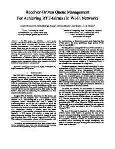
does forward-backward searching for the optimal control solution. Let us choose an initial control trajectory: (𝑢0 , . . . , 𝑢𝑁), (𝛿𝑢0 , . . . , 𝛿𝑢𝑁); (𝑢+0 = 𝑢0 , . . . , 𝑢+𝑁 = 𝑈𝑁); 𝐽− = ∞, 𝛾, Iter = 1, Δ 0 , TOL, MaxIter, 𝜌 ∈ [0, 1]. From Algorithm 1 (FB-OCQ), it is obvious that the algorithm terminates if the norm of the gradient of the Hamiltonian with respect to 𝑢, 𝛾 = ‖𝐻𝑢 ‖2 , during the run time of the program, is smaller than the tolerance and the parameter 𝛽 must change at the inner iterations if we do not have a descent direction, so we must divide 𝛽 by parameter 𝜌 ∈ (0, 1) until we get a reduction in the cost function. Figure 2 explains our algorithm steps: forward sweep (control variable and cost function value) and backward sweep (adjoint variable) in detail.
6
Scientific Programming t0
Forward sweep
tf
t1
u = u + 𝛿u J+ = 1 < J− = ∞ → J− = J+ = 1 Decrease 𝛽 J+ = 2 > J− = 1
x(t), u(t)
Backward sweep
Increase 𝛽 J = 0.5 < J = 1 + − → J− = J+ = 0.5
Figure 2: FB-OCQ algorithm explanation.
60 50 40 30 20 10 0 0.0
0.5
1.0 Time (sec)
1.5
2.0
60 50 40 30 20 10 0 0.0
0.5
1.0 Time (sec)
1.0 Time (sec)
1.5
2.0
1.5
2.0
Actual input rate u(t)
Actual input rate u(t)
6 5 4 3 2 1 0 0.0
0.5
1.5
2.0
Average buffer load x(t)
Figure 3: Indirect method: FB-OCQ.
5. Performance Evaluation 5.1. Numerical Results. In this section, we provide some iteration results for both direct and indirect approaches as follows. Indirect Method: FB-OCQ. The ODE was solved on equidistant discretization with 1000 discretization points. The optimal control and optimal state are depicted in Figure 3. We realize, by looking at the final control, that there exist some points where the set of active constraints changed due to the singularity; that is, the optimal control is of the bang-bang type with the possibility of a singular arc. To the meaning of such singular arc for queue management, it presents the sudden changes of input rate from 60 (packets/sec) to 35 (packets/sec) which accordingly result in the changes of buffer load (or queue length). In the 𝛽 history, in Figure 3, the parameter 𝛽 changed at the inner iterations because we do not have a descent direction, so we must divide 𝛽 by 𝜌 ∈ (0, 1) until we get a reduction in the cost function J = 6.81280316. The processing time of central processing unit (CPU) for this algorithm is 0.04 s and the norm of the gradient of
6 5 4 3 2 1 0 0.0
0.5
1.0 Time (sec)
Average buffer load x(t)
Figure 4: Direct method: nonlinear optimization with JModelica solver.
the Hamiltonian function ‖𝐻𝑢 ‖2 with respect to the control 𝑢 goes to approximately 10𝑒 − 7. Direct Collocation Method: JModelica and GAlib Solvers. With 𝑁 = 1000 and the number of interpolation points being 3, we tested the discretized problem (9)-(10) by JModelica and GAlib solvers (see [20, 21]) as follows. (i) JModelica Solver. The cost function is reduced to J = 6.8678362 and the CPU processing time is 0.52 s. The optimal control and optimal state trajectories are obtained during JModelica running and illustrated in Figure 4. An advantage of this approach is that we do not need to derive the adjoint equations. (ii) GAlib Solver. For this problem, we use the number of generations 𝑛gen = 2500, and the population size is 200. The optimal control and optimal state are depicted in Figure 5 obtained during the run of the GAlib. The cost function is reduced to J = 7.06744 during the run time of the program. The CPU processing time is 1.290 s. Although the genetic
Scientific Programming 60 50 40 30 20 10 0 0.0
7 .. . Source 1
Source 2
0.5
1.0 Time (sec)
1.5
2.0
.. .
Router
Destination
Actual input rate u(t)
6 5 4 3 2 1 0 0.0
Source 40
Figure 6: Simulation topology. 0.05 1.0
0.5
1.5
2.0
0.04
Average buffer load x(t)
Figure 5: Direct method: genetic algorithm with GAlib solver. Table 1: Numerical result summary. Criteria/methods Cost function value CPU process time
Direct GAlib
Direct JModelica
Indirect FB-OCQ
J = 7.067 1.29 (sec)
J = 6.867 0.52 (sec)
J = 6.812 0.04 (sec)
algorithm has an advantage that it needs no derivatives or Hessian’s information, the control functions produced by it are useless and the convergence is very slow in comparison to Algorithm 1 (FB-OCQ) and the one using JModelica solver. Table 1 summarizes and compares the three methods that we develop numerically. We conclude that Algorithm 1 is much faster than the other solvers and gives the best cost function. By using genetic library GAlib, the cost function does not reach the local solution as it claims in finding the global solution. The limitation of the indirect methods (FBOCQ) is that one should derive the adjoint equations which are not easy to derive in some applications. 5.2. Simulation Results. In this section, the performance of the obtained algorithm (FB-OCQ) is evaluated by comparing it with some popular AQMs including RED, REM, and PI. The credibility of results is confirmed using ns-2 simulator [24]. We investigate a network topology with 40 sources, an intermediate router, and one destination (Figure 6). All sources simultaneously send packets to the destination through the router. Hence, a large queue is built up at the router or bottleneck point. Maximum buffer size of the router is 100 packets. All of the compared RED, REM, and PI algorithms are configured to obtain the desired queue length at 40 packets. Simulation lasts for 60 seconds and is repeated using a built-in random generator in ns-2 to obtain more credible results.
Dropping probability
Time (sec) 0.03
0.02
0.01
0.00
0
10
20
30 Time (sec)
40
50
60
FB-OCQ RED
Figure 7: Dropping probability.
Figure 7 shows dropping probability of FB-OCQ and RED algorithms. With the proposed square-root drop function, FB-OCQ drops queuing packets more aggressively than RED although dropping frequency is nearly the same. Maximum dropping ratio is 0.045 for FB-OCQ and 0.039 for RED. In fact, when the algorithm drops more packets, the queue stability will be increased but we will have to sacrifice the system throughput performance. We can see this trade-off in next results. Figure 8 presents average queue length values measured at the bottleneck link from router to destination for different algorithms. Due to aggressive dropping, FB-OCQ maintains the shortest queue at 40 packets which is also the desired value. Only REM can obtain the same value but in a longer time, ≈50 seconds. PI, in fact, can achieve the same performance only if its parameters are well configured and be dynamically changed to different network scenarios. In Figure 8, we can see that PI performs not so well, even we set the desired queue length variable at 40 packets and exploit default parameters in ns-2 for PI controller. Finally, we investigate throughput performance of proposed FB-OCQ algorithm. It is confirmed from Figure 9 that there exists a trade-off in the relationship between
8
Scientific Programming 70
Average queue length (packets)
Experiment: 60
DropTail
50 40
RED FB-OCQ
30
Figure 10: Experiment test setup, from the test client to the test server.
20 10 0
0
10
20
30 Time (sec)
40
50
60
REM PI
FB-OCQ RED
Figure 8: Average queue length versus time. 0.09 0.08 0.07 Throughput (Mbps)
Bufferbloat server
0.06 0.05 0.04 0.03 0.02 0.01 0.00
FB-OCQ
RED
REM
PI
Figure 9: Throughput comparison.
throughput and queue length/dropping probability. PI and REM achieve nearly the same throughput at 0.06 (Mbps) while FB-OCQ and RED obtain the better throughput performance at 0.08 (Mbps) value. In Figure 8, although REM can achieve the desired queue length 40 packets in this scenario, REM still maintains a large queue during simulation time from 0 (sec) up to 25 (sec). That reason leads to throughput performance of REM being lower than RED and FB-OCQ. Our proposed FB-OCQ drops aggressively the packets so that its throughput value (0.075904 Mbps) is slightly less than RED (0.082146 Mbps). 5.3. Experiment Results. We examine the effectiveness of our state-of-the-art optimal control queue method in the Linux kernel (e.g., Ubuntu 16.04). We conduct experiment from a desktop computer through the Internet gateway to an outside server (Figure 10). To manage working queuing disciplines (qdiscs), we use the scheduler qdisc in the Linux kernel. The chosen server is a dedicated bufferbloat server,
which is able to stand very high congestion due to many data flows at the same time. We exploit the Flent: FLExible Network Tester [25] and Realtime Response Under Load (RRUL) test [26] to evaluate our proposal. RRUL test puts a network under worst case conditions, reliably saturates the network link, and thus recreates bufferbloat phenomenon for queue algorithm testing. Simulation time duration is 60 seconds. We compare latency under load test with queue being handled by different AQM schemes (DropTail, RED, and FBOCQ) in turn. DropTail queuing method is by far the simplest approach to network router queue management. The router accepts and forwards all the packets that arrive as long as its buffer space is available for the next incoming packets. If a packet arrives and the queue is currently full, the incoming packet will be dropped. The sender then detects the packet lost event and shrinks its sending window. While it is the most widely used due to simplicity and relatively high efficiency, DropTail has some weakness such as the bad fairness sharing among TCP connections, and throughput and bottleneck link efficiency suffer severe degradation if congestion is getting worse. RED [5, 6] was presented with the objective of minimizing packet loss and queuing delay. Moreover, it can compensate the weakness of DropTail by avoiding global synchronization of TCP sources so that it improves fairness. To achieve these goals, RED utilizes two thresholds, minth and maxth , and an exponentially weighted moving average (EWMA) formula to estimate average queue length [27]. When the average queue length exceeds a predefined threshold, the link is implied to be in congested state and drop action is taken. A temporary increase in the queue length notifies the transient congestion, while an increase in the average queue length reflects long-lived congestion. Based on such information, RED router sends randomized feedback signals to the senders to make decision of decreasing their congestion windows. RED has good fairness among connections because of the feedback randomized mechanism [28]. Figure 11 presents latency ping results under RRUL test suite. Ping is a networking utility and operates by sending Internet Control Message Protocol (ICMP) echo request packets to the target server and waits for an ICMP echo reply. The program measures the round-trip time from transmission to reception, reporting errors and packet loss. Our proposed algorithm FB-OCQ achieves the lowest packet latency compared with the other two algorithms inside Linux
Packet latency (ms)
Scientific Programming
9 [3] J. Gettys, “Bufferbloat: views of the elephant,” in Proceedings of the International Summit for Community Wireless Networks, October 2012.
103
[4] B. Braden, D. Clark, J. Crowcroft et al., “Recommendations on queue management and congestion avoidance in the internet,” RFC 2309, IETF, San Francisco, Calif, USA, 1998.
102
101 0
10
20
30
40
50
60
Simulation time (s) DropTail RED FB-OCQ
[5] C. Hollot, V. Misra, D. Towsley, and W.-B. Gong, “A control theoretic analysis of red,” in Proceedings of the 20th Annual Joint Conference of the IEEE Computer and Communications Societies (INFOCOM ’01), vol. 3, pp. 1510–1519, IEEE, Anchorage, Alaska, USA, 2001. [6] S. Floyd and V. Jacobson, “Random early detection gateways for congestion avoidance,” IEEE/ACM Transactions on Networking, vol. 1, no. 4, pp. 397–413, 1993.
Figure 11: ICMP ping result using Realtime Response Under Load test.
[7] S. Athuraliya, S. Low, and D. Lapsley, “Random early marking,” in Quality of Future Internet Services, J. Crowcroft, J. Roberts, and M. I. Smirnov, Eds., vol. 1922 of Lecture Notes in Computer Science, pp. 43–54, Springer, Berlin, Germany, 2000.
kernel. Specifically, the packet latency when using FB-OCQ is about 80 (ms), while about 120 (ms) if using DropTail (pfifo fast in Ubuntu) and 100 ms if using RED algorithm.
[8] R. Pan, P. Natarajan, C. Piglione et al., “PIE: a lightweight control scheme to address the bufferbloat problem,” in Proceedings of the IEEE 14th International Conference on High Performance Switching and Routing (HPSR ’13), pp. 148–155, Taipei, Taiwan, July 2013.
6. Conclusions We proposed a queue management algorithm named forward-backward optimal control queue (FB-OCQ) to solve the OCQ problem. Derived from indirect approaches in dynamic optimization, this algorithm demonstrates faster reaction while still achieving the same performance in numerical analysis compared to direct methods. Employing under network simulation ns-2, we see that the proposed algorithm drops packets more aggressively than the traditional RED algorithm, in a higher frequency and magnitude. As a result, average queue length can be reduced much more, while an acceptable value of throughput still can be maintained. In future works, we try to investigate the memory efficiency of FB-OCQ under wireless sensor networks.
Competing Interests The authors declare that there is no conflict of interests regarding the publication of this paper.
Acknowledgments This work was supported by the National Research Foundation of Korea (NRF) grant funded by the Korean government (MEST) (no. NRF-2016R1A2B1013733).
References [1] T. Hoiland-Jorgensen, “Battling bufferbloat: an experimental comparison of four apapproach to queue management in linux,” Tech. Rep., Roskilde University, Roskilde, Denmark, 2012. [2] J. Gettys, “Bufferbloat: dark buffers in the Internet,” IEEE Internet Computing, vol. 15, no. 3, pp. 95–96, 2011.
[9] F. Ren, C. Lin, and B. Wei, “Design a robust controller for active queue management in large delay networks,” in Proceedings of the 9th International Symposium on Computers and Communications (ISCC ’04), vol. 2, pp. 748–754, June-July 2004. [10] R. Zhu, H. Teng, and J. Fu, “A predictive PID controller for AQM router supporting TCP with ECN,” in Proceedings of the 5th International Symposium on Multi-Dimensional Mobile Communications. The 2004 Joint Conference of the 10th AsiaPacific Conference on Communications, vol. 1, pp. 356–360, August-September 2004. [11] J. Sun, M. Zukerman, and M. Palaniswami, “Stabilizing RED using a fuzzy controller,” in Proceedings of the IEEE International Conference on Communications (ICC ’07), pp. 266–271, Glasgow, Scotland, June 2007. [12] H.-L. To, T. M. Thi, and W.-J. Hwang, “Cascade probability control to mitigate bufferbloat under multiple real-world TCP stacks,” Mathematical Problems in Engineering, vol. 2015, Article ID 628583, 13 pages, 2015. [13] M. Hassan and H. Sirisena, “Optimal control of queues in computer networks,” in Proceedings of the International Conference on Communications (ICC ’01), vol. 2, pp. 637–641, June 2001. [14] V. Guffens and G. Bastin, “Optimal adaptive feedback control of a network buffer,” in Proceedings of the American Control Conference (ACC ’05), vol. 3, pp. 1835–1840, Portland, Ore, USA, June 2005. [15] J. T. Betts, Practical Methods for Optimal Control Using Nonlinear Programming, Society for Industrial and Applied Mathematics, Philadelphia, Pa, USA, 2001. [16] R. Bulirsch, E. Nerz, H. Pesch, and O. von Stryk, “Combining direct and indirect methods in optimal control: Range maximization of a hang glider,” in Optimal Control, R. Bulirsch, A. Miele, J. Stoer, and K. Well, Eds., vol. 111 of ISNM International Series of Numerical Mathematics, pp. 273–288, Birkhuser, Basel, Switzerland, 1993. [17] A. Radwan, Utilization of parametric programming and evolutionary computing in optimal control [Ph.D. dissertation], Humboldt-Universit¨at zu Berlin, 2012.
10 [18] O. von Stryk and R. Bulirsch, “Direct and indirect methods for trajectory optimization,” Annals of Operations Research, vol. 37, no. 1, pp. 357–373, 1992. [19] A. Bryson and Y. Ho, Applied Optimal Control: Optimization, Estimation and Control, Hemisphere: CRC Press, Washington, DC, USA, 1975. [20] M. Ab, Jmodelica.org user guide 1.6.0, 2011, http://www.jmodelica.org/page/236. [21] M. Wall, GAlib: A C++ Library of Genetic Algorithm Components, Version 2.4 Documentation Revision B, Massachusetts Institute of Technology, 1996. [22] A. Radwan, O. Vasilieva, R. Enkhbat, A. Griewank, and J. Guddat, “Parametric approach to optimal control,” Optimization Letters, vol. 6, no. 7, pp. 1303–1316, 2012. [23] J. Guddat, F. Guerra Vazquez, and H. T. Jongen, Parametric Optimization: Singularities, Pathfollowing and Jumps, John Wiley & Sons, 1990. [24] T. Issariyakul and E. Hossain, Introduction to Network Simulator NS2, Springer, Berlin, Germany, 1st edition, 2008. [25] T. Hiland-Jrgensen, Flent: The flexible network tester, 2012– 2015, https://flent.org. [26] D. Tht, “Realtime response under load (rrul) test,” 2013, https:// github.com/dtaht/deBloat/blob/master/spec/rrule.doc. [27] J. Koo, S. Ahn, and J. Chung, “A comparative study of queue, delay, and loss characteristics of AQM schemes in QoS-enabled networks,” Computing and Informatics, vol. 23, no. 4, pp. 317– 335, 2004. [28] T. B. Reddy and A. Ahammed, “Performance comparison of active queue management techniques,” Journal of Computer Science, vol. 4, no. 12, pp. 1020–1023, 2008.
Scientific Programming
Journal of
Advances in
Industrial Engineering
Multimedia
Hindawi Publishing Corporation http://www.hindawi.com
The Scientific World Journal Volume 2014
Hindawi Publishing Corporation http://www.hindawi.com
Volume 2014
Applied Computational Intelligence and Soft Computing
International Journal of
Distributed Sensor Networks Hindawi Publishing Corporation http://www.hindawi.com
Volume 2014
Hindawi Publishing Corporation http://www.hindawi.com
Volume 2014
Hindawi Publishing Corporation http://www.hindawi.com
Volume 2014
Advances in
Fuzzy Systems Modelling & Simulation in Engineering Hindawi Publishing Corporation http://www.hindawi.com
Hindawi Publishing Corporation http://www.hindawi.com
Volume 2014
Volume 2014
Submit your manuscripts at http://www.hindawi.com
Journal of
Computer Networks and Communications
Advances in
Artificial Intelligence Hindawi Publishing Corporation http://www.hindawi.com
Hindawi Publishing Corporation http://www.hindawi.com
Volume 2014
International Journal of
Biomedical Imaging
Volume 2014
Advances in
Artificial Neural Systems
International Journal of
Computer Engineering
Computer Games Technology
Hindawi Publishing Corporation http://www.hindawi.com
Hindawi Publishing Corporation http://www.hindawi.com
Advances in
Volume 2014
Advances in
Software Engineering Volume 2014
Hindawi Publishing Corporation http://www.hindawi.com
Volume 2014
Hindawi Publishing Corporation http://www.hindawi.com
Volume 2014
Hindawi Publishing Corporation http://www.hindawi.com
Volume 2014
International Journal of
Reconfigurable Computing
Robotics Hindawi Publishing Corporation http://www.hindawi.com
Computational Intelligence and Neuroscience
Advances in
Human-Computer Interaction
Journal of
Volume 2014
Hindawi Publishing Corporation http://www.hindawi.com
Volume 2014
Hindawi Publishing Corporation http://www.hindawi.com
Journal of
Electrical and Computer Engineering Volume 2014
Hindawi Publishing Corporation http://www.hindawi.com
Volume 2014
Hindawi Publishing Corporation http://www.hindawi.com
Volume 2014