Optimal Control of Complex Systems Based on Improved Dual
Recommend Documents
SWITCHED systems are a particular class of hybrid sys- tems that consist of ... real-world processes such as chemical processes, automotive systems, and .... optimal control methods, but also nonlinear optimization tech- niques. ...... [15] B. Lincol
solving optimal control problems for switched systems. ... The optimal control problem is there by ..... [10] B. Lincoln, B. M. Bernhardsson, Efficient pruning.
Nov 28, 2012 - synchronized regions with temporal period 2 emerge from random initial conditions. ..... New ways to find solutions to the control problem that do not intend to ..... Table 2.2: Notation used to define an agent-based simulation.
May 9, 2018 - Keywords: multi-rate systems; optimization; aperiodic control; ... In the algorithm we maximize the decay rate of the system after a full sampling ...
valued analysis, these systems have not been closely studied either .... problem (that is, it does not depend on the other parameters introduced, ... For θ < 1, the main problem is one of âchatteringâ: the numerical solutions will ...... [35] R.
Chih-Ming Ho and Pak Kin Wong. Institute for Cell Mimetic Space Exploration and. Mechanical and Aerospace Engineering Department,. University of California ...
attractors. associated either with maps or first order ordinary differential equations (ODE) in R n. The control is ...
Aug 31, 2014 - on this model, the dynamic programming optimal control strategy is employed to design controller for every initial cell. In spite of optimal control ...
Exploration and Mechanical and Aerospace Engineering Department,. University of California, Los Angeles, CA 90095 USA (e-mail: [email protected] ...
development of bioprocess engineering including monitoring of product ... Control of engineering systems has been conducted in several areas ... are more susceptible to local optimum solutions rather than ..... which is essential for making of alcoho
come in the form of fifth-order polynomial equations (in the unknown ...... [16] R. L. Raffard, C. J. Tomlin, and S. Boyd, âDistributed optimization for cooperative ...
front wheel vibration signals to adjust the characteristics of rear suspension. But in practice, the road disturbance information is difficult to be measured due to ...
It has been proved [15] that closed-loop stability of the MPC controller is guaranteed by .... 3 Design of stabilizing MPC based on saturating control laws ..... 0 0.5. 1 0.5.... where the inputs are constrained to uâ ⤠0.3 and xâ ⤠2.
Cuong Cao1, Le Ly Thuy Tram1, Anders Wolff2 and Dang Duong Bang1* .... X. X. Li, C. Cao, S. J. Han and S. J. Sim, Water Res., 2009, 43, 1425-1431. 6.
Jun 5, 2009 - linear controllers for wind energy systems, and the book highlights several of .... U.S. National Renewable Energy Laboratory [11]. The book ...
This HVAC system is made of two heat exchangers: an air-to-air heat exchanger (a rotary wheel heat recovery) and a water-to- air heat exchanger. First dynamic ...
Lei Liu. 1 and Wanquan Liu. 2. 1School of Electrical Engineering and ... As we know, the LQ optimal control problem can be transformed into a problem of.
Email: [email protected]. Summary. This study extensively addresses the application of optimal control approach to the automatic generation control (AGC) of ...
WindRiver Systems corporation, which offers POSIX 1003.1b real-time UNIX extensions and analysis opportunities like process schedule monitoring and other ...
This paper has been digitized, optimized for electronic delivery and stamped with · digital signature within the project DML-CZ: The Czech Digital Mathematics ...
and subdifferentiable there. Due to the continuity of F*(0, -)over V*, its maximiza tion may be performed over any space dense in V* so that e.g. the problem (3") ...
Abstract: Dual-complex Fibonacci numbers with Fibonacci and Lucas coefficients are introduced ... In this paper, we define dual-complex numbers by using the.
Jan 4, 2010 - c California Institute of Technology. All rights reserved. This manuscript is for review purposes only and may not be reproduced, in whole or in.
Optimal Control of Complex Systems Based on Improved Dual
Aug 27, 2017 - solve the optimal control problem, the âcurse of dimension- alityâ problem, so ... of HDP, and the control effect of the HDP structure needed improvement [17] ...... and summarized the effects of evaporation temperature, distance, and .... systems which have features such as multiple variables, strong coupling ...
Hindawi Mathematical Problems in Engineering Volume 2017, Article ID 5476415, 11 pages https://doi.org/10.1155/2017/5476415
Research Article Optimal Control of Complex Systems Based on Improved Dual Heuristic Dynamic Programming Algorithm Hui Li,1,2 Yongsui Wen,1 and Wenjie Sun1 1
School of Electrical and Electronic Engineering, Changchun University of Technology, Changchun, China Jilin University, Changchun, China
1. Introduction With the increase of the dynamic complexity of controlled objects and their widespread application, some dynamic models of controlled objects can be obtained by mathematical methods. But some of the controlled objects are too complex to establish an accurate mathematical model, such as a robot system and a chemical generation process. Even though the mathematical model of complex systems has been established, it will be usually a high-order nonlinear time-varying complex differential equation. So, it could not describe the system accurately, and it is too difficult to analyze and process the data, and hence the unknown model must be learned by the observational data [1]. This is because of the great fault tolerance, self-adaptation, self-organization, and learning and memory ability of neural networks, which provides a new method for the modeling of complex systems [2–5]. However, BP networks, RBF networks, and SVM have some defects such as slow convergence, which causes a big gap between the approximation ability and the actual demand of complex systems [6, 7]. In order to solve this problem, Huang GB proposed single hidden layer feedforward network (SLFN)
training—Extreme learning Machine (ELM)—in 2006 [8]. The ELM gives the weights and thresholds of the weights randomly and then calculates the output weights by the regularization principle, which can still approach any continuous system [6, 7]. It has been proved that the SLFN hidden layer node parameter randomly accessed does not affect the convergence ability, and it also makes the speed of learning the ELM thousands of times faster than the traditional BP network and SVM. In recent years, dynamic programming has been used to solve the optimal control problem, the “curse of dimensionality” problem, so no optimal solution could be obtained [9]. In 1977, Werbos proposed a heuristic dynamic programming (HDP) and dual heuristic programming (DHP) concept and proposed a method of approximate dynamic programming (adaptive/approximate dynamic programming, ADP) to solve the “curse of dimensionality” problem [10]. Werbos defines “intelligence” as the brain’s ability to learn a utility function maximally in a complex, unknown, nonlinear environment [11]. ADP is the general scheme for learning approximate optimal action strategies. Therefore, ADP can be regarded as a key method which is able to design the
2
Mathematical Problems in Engineering
Critic network
x(k)
u(k) Action network
Model network
x (k + 1)
Critic network
J [x (k)] x (k)
J [x (k + 1)] x (k + 1)
−
+
[(x (k), u (k))] x (k)
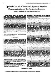
Figure 1: The structural diagram of the DHP algorithm.
intelligent system of a brain. According to the basic principle, realization structure, and current development of the ADP method, Lewis and others gave a summary and prospect of the research and pointed out that ADP is an effective datadriven method [12–15]. ADP can realize the optimization control of the nonlinear system by using neural networks based on online data and control information to approximate the performance index function of the optimal control law, without a mathematical model of a nonlinear control system [16]. To develop neural dynamic programming results and relax the system dynamic requirements, Zhong et al. proposed a new goal representation ADP online optimization control structure for nonlinear systems. But the network could not output the derivative function information of the cost function directly based on the implementation structure of HDP, and the control effect of the HDP structure needed improvement [17]. In fact, some studies show that DHP and GDHP can be controlled better than HDP in the structure of ADP method to some extent [18, 19]. In general, the study on the optimal control of nonlinear systems of ADP based on the traditional neural network has made great progress. But the ADP still has problems of slow response and poor stability. In this paper, ELM algorithm gives random input weights and thresholds to improve the response speed of the DHP algorithm and the stability of the DHP algorithm is improved by calculating the output weights by the regularization principle. In order to verify the validity of the algorithm, the ELM-DHP was designed to control the molecular distillation system with multivariability, nonlinearity, strong coupling, and large delay.
2. Algorithm Principle 2.1. DHP Algorithm Principle. The discrete-time nonlinear dynamic system is described as follows: 𝑥 (𝑘 + 1) = 𝐹 [x (𝑘) , u (𝑘) , 𝑘] ,
𝑘 = 0, 1, . . . .
(1)
In formula (1), x(𝑘) ∈ R𝑛 represents the state vector of the system, u(𝑘) ∈ R𝑛 represents control variables, and 𝐹 represents the system function.
The performance index function (also called the cost function) corresponding to the system is ∞
𝐽 [x (𝑘) , 𝑘] = ∑𝛾𝑖−𝑘 𝜂 [x (𝑖) , u (𝑖) , 𝑖] ,
(2)
𝑖=𝑘
where 𝜂 is the utility function, 𝛾 is the discount factor (0 < 𝛾 ≤ 1), 𝐽 is the cost function of state x(𝑘), and 𝐽 depends on the initial time 𝑘 and the initial state x(𝑘). For DHP, the purpose of dynamic programming is to select a control sequence u(𝑖), 𝑖 = 𝑘, 𝑘 + 1, . . . , 𝑙, which minimizes the function 𝜕𝐽[x(𝑘)]/𝜕x(𝑘). The DHP structure is shown in Figure 1, which contains three neural networks: model network, critic network, and action network. The neural network has a powerful function of universal approximation, so the model network can be used to model the unknown nonlinear or complex nonlinear system and make the DHP method widely used. The input of the critic network is a state variable. The output of the critic network is approximation performance index function J on the state x derivative, which is also known as the costate. The action network, also known as “Actor,” represents the mapping between system state variables and control variables [20–22]. 𝜕𝐽[x(𝑘)]/𝜕x(𝑘) is based on the iteration of the derivative for performance index function and utility function to state. 𝜕𝐽 [x (𝑘)] 𝜕𝜂 {x (𝑘) , u [x (𝑘)]} 𝜕𝐽 [x (𝑘 + 1)] = +𝛾 . 𝜕x (𝑘) 𝜕x (𝑘) 𝜕x (𝑘)
(3)
In (3), u[x(𝑘)] is a feedback control variable, and costates 𝜕𝐽[x(𝑘)]/𝜕x(𝑘) and 𝜕𝐽[x(𝑘 + 1)]/𝜕x(𝑘) are the outputs of the critic network. If the weight of the critic network is set to 𝜔, the right type of formula (1) is set to 𝑒 [x (𝑘) , 𝜔] =
At the same time, the left type of formula (1) can be written as 𝜕𝐽[x(𝑘), 𝜔]/𝜕x(𝑘). By adjusting the weights 𝜔 of
Mathematical Problems in Engineering
3
the critic network, the least-mean-square-error function is as follows: 𝜕𝐽 [x (𝑘) , 𝜔] 2 { 𝜔∗ = arg min − 𝑒 , 𝜔] (𝑘) [x } . 𝜕x (𝑘) 𝜔
(5)
According to the principle of optimality, the optimal control should satisfy the first-order differential necessary condition. 𝜕𝐽∗ [x (𝑘)] 𝜕𝜂 [x (𝑘) , u (𝑘)] 𝜕𝐽∗ [x (𝑘 + 1)] = + 𝜕u (𝑘) 𝜕u (𝑘) 𝜕u (𝑘) 𝜕𝜂 [x (𝑘) , u (𝑘)] = 𝜕u (𝑘) +
(6)
(7)
∗
In formula (7), 𝜕𝐽 [x(𝑘 + 1)]/𝜕x(𝑘 + 1) is the optimal costate, satisfying formula (5). From (1) to (7), we can conclude that the optimal control quantity of the DHP method can be obtained directly by the costate. Compared with the HDP method which obtained the optimal control by the relationship between the weights (𝜔) of the critic network and the input–output, the method of DHP has more computational efforts, but better control effect [9]. 2.2. ELM Algorithm Principle. For a standard SLFN with 𝐿 hidden layer neurons learning 𝑁 arbitrary distinct samples (x𝑗 , t𝑗 ), x𝑗 = [𝑥𝑗1 , 𝑥𝑗2 , . . . , 𝑥𝑗𝑛 ]𝑇 ∈ 𝑅𝑛 , t𝑗 = [𝑡𝑗1 , 𝑡𝑗2 , . . . , 𝑡𝑗𝑚 ]𝑇 ∈ 𝑅𝑚 and activation function 𝑔(⋅) are mathematically modeled as [23] 𝐿
𝑖=1
(8)
𝑗 = 1, 2, . . . 𝑁, 𝑏𝑖 , 𝛽𝑖 ∈ 𝑅, 𝑎𝑖 ∈ 𝑅, where o𝑗 = [𝑜𝑗1 , 𝑜𝑗2 , . . . , 𝑜𝑗𝑚 ]𝑇 ∈ 𝑅𝑚 is the model output of the network, w𝑖 = [𝑤𝑖1 , 𝑤𝑖2 , . . . , 𝑤𝑖𝑛 ]𝑇 is the input weight matrix between the input layer neuron and the 𝑖th hidden layer neuron, 𝛽𝑖 is the output weight matrix between the 𝑖th hidden layer neuron and the output layer neurons, 𝑏𝑖 is the threshold of the 𝑖th neuron in the hidden layer, and w𝑖 ⋅ x𝑗 is the inner product of w𝑖 and x𝑗 . The learning objective of the SLFN is to minimize the output error. Error can be expressed as 𝑁 ∑ t𝑗 − o𝑗 = 0.
𝑗=1
(10)
𝑖=1
So, (10) can be written as H𝛽 = T, where H (w1 , . . . , w𝐿 , 𝑏1 , . . . , 𝑏𝑁, x1 , . . . , x𝑁) 𝑔 (w1 ⋅ x1 + 𝑏1 ) ⋅ ⋅ ⋅ 𝑔 (w𝐿 ⋅ x1 + 𝑏𝐿 ) ⋅⋅⋅
t𝑇1 [ ] [ ] . T = [ ... ] [ ] 𝑇 [t𝑁]𝑁×𝑚 H is a hidden layer output matrix of ELM. So, the training ̂ of linear of ELM is equivalent to the least-squares solution 𝛽 system H𝛽 = T. H (̂ ̂ − T = min H (̂ ̂ w𝑖 , ̂𝑏𝑖 ) 𝛽 (12) w,𝑏,𝛽 w𝑖 , 𝑏𝑖 ) ⋅ 𝛽 − T . In (12), 𝑖 = 1, 2, . . . , 𝐿, (12) is equivalent to minimizing the loss function 2 𝑁 𝐿 (13) 𝐸 = ∑ ∑𝛽𝑖 ⋅ 𝑔 (w𝑖 ⋅ x𝑗 + 𝑏𝑖 ) − t𝑗 . 𝑖=1 𝑗=1 Huang et al. [23] proved that the minimum value of the least-squares solution of the linear system satisfies the following. ̂ = H−1 T (1) Minimum Training Error. The special solution 𝛽 is one of the least-squares solutions of a general linear system H𝛽 = T,H−1 which is a generalized inverse matrix of H. (2) Smallest Norm of Weights and Best Generalization Capâ = H−1 T has the smallest bility. Further, the special solution 𝛽 norm among all of the least-squares solutions of H𝛽 = T : ̂ = ‖H−1 T‖ ≤ ‖𝛽‖, ∀𝛽 ∈ {𝛽 : ‖H𝛽 − T‖ ≤ ‖Hz − T‖, ∀z ∈ ‖𝛽‖ R𝑁×𝑁}. The generalization ability of SLFN with minimum weight is independent of the number of parameters [24]. The smaller the weight, the stronger the generalization ability of SLFN. (3) Special Solution. The least-squares solution of H𝛽 = T is unique. 2.3. Proof the Stability of ELM-DHP. The stability of the ELM-DHP algorithm is proved (i.e., the output error of the system is 0). The discrete nonlinear system is controlled
4
Mathematical Problems in Engineering x1 (k)
The model network is trained offline, and the calculation process is as follows. The input layer to the hidden layer weight matrix W𝑚1 and the hidden layer threshold matrix B = [𝑏1 , 𝑏2 . . . , 𝑏𝑙𝑚 ] are randomly generated. Define the input vector M(𝑘) and the expected output vector x̂(𝑘) of the model network in 𝑘 moments:
by the ELM-DHP algorithm, and the three networks of the ELM-DHP algorithm are all based on the fixed ELM implementation. Therefore, it just needs to be proved that ELM can approximate the discrete nonlinear system by 0 error. The ELM learning algorithm is chosen as a SLFN with 𝐿 hidden layer neurons. The 𝑁 arbitrary distinct samples (x𝑗 , t𝑗 ), where 𝐿 ≤ 𝑁, x𝑗 = [𝑥𝑗1 , 𝑥𝑗2 , . . . , 𝑥𝑗𝑛 ]𝑇 ∈ 𝑅𝑛 , and t𝑗 = [𝑡𝑗1 , 𝑡𝑗2 , . . . , 𝑡𝑗𝑚 ]𝑇 ∈ 𝑅𝑚 of the nonlinear discrete system and nonlinear activation function 𝑔(⋅), are mathematically modeled as formula (8). ELM learns a large number of samples generally, and the number of neurons in the hidden layer is far less than the number of samples, 𝐿 ≪ 𝑁. So, we only need to prove that the learning error of ELM was 0 when 𝐿 ≤ 𝑁. Huang et al. [7, 23, 25] proved in detail that the SLFN with 𝐿 neurons can approximate any arbitrary sample (x𝑗 , t𝑗 ) at any small error; that is,
where 𝑚ℎ1𝑗 (𝑘) is the input of the 𝑗th node in the model network hidden layer, 𝑚ℎ2𝑗 (𝑘) is the output of the 𝑗th node in the model network hidden layer, and mℎ2 = [𝑚ℎ21 , 𝑚ℎ22 , . . . , 𝑚ℎ2𝑙𝑚 ] ∈ 𝑅𝑚 . Calculate the weights W𝑚2 (𝑘) from the hidden layer to the output layer: x̂ (𝑘 + 1) = mℎ2 (𝑘) × W𝑚2 (𝑘) .
(17)
According to the idea of the ELM, the error is minimized
Calculate the output matrix mℎ2 (𝑘) of the hidden layer in the model network
(14)
𝑗=1
The work above proves that the learning error of ELM is 0 (i.e., the stability of the ELM-DHP algorithm).
3. Implementation of the ELM-DHP Algorithm The ELM-DHP algorithm includes three networks: model network, critic network, and action network. The hidden layer of the three networks is a sigmoidal bipolar function and the output layer is a purelin linear function. The realization process of the ELM-DHP algorithm is studied by using the discrete-time nonlinear dynamic programming of 𝑛dimensional state vector and 𝑚-dimensional control vector as the research object. 3.1. Network Model. The model network adopts (𝑚+𝑛)−𝑙𝑚 −𝑛 structure. The 𝑚 + 𝑛 inputs are the 𝑛 components of the state vector x(𝑘) in the 𝑘 moments and the 𝑚 components of the predicted output u(𝑘) of the action network to state x(𝑘) in the system of (𝑘 − 1) moments. The 𝑛 output is the 𝑛 components of the prediction vector x̂(𝑘 + 1) to the state vector x(𝑘 + 1) in the system of (𝑘 + 1) moments. The model network has 𝑙𝑚 hidden layer neurons. The structure of the model network is shown in Figure 2.
In equality (18), 𝑥𝑖 (𝑘 + 1) is the expected output 𝑖th output layer neurons of the model network. W𝑚2 (𝑘) is equivalent to solving the least-squares solution ̂ 𝑚2 (𝑘) of the linear system mℎ2 (𝑘) × W𝑚2 (𝑘) = x̂(𝑘 + 1): W ̂ 𝑚2 − x̂ (𝑘 + 1) mℎ2 (𝑘) × W = min mℎ2 (𝑘) × W𝑚2 − x̂ (𝑘 + 1) . W𝑚2
(19)
̂ 𝑚2 (𝑘) of the weight matrix of the The special solution W hidden layer and output layer in the model network is as follows: ̂ 𝑚2 (𝑘) = m−1 (𝑘) × x̂ (𝑘 + 1) , W ℎ2
(20)
where m−1 ℎ2 (𝑘) is a generalized inverse matrix of mℎ2 (𝑘) in 𝑘 moments. 3.2. Critic Network. The critic network is composed of 𝑛 − 𝑙𝑐 − 𝑛. The 𝑛 inputs are the 𝑛 components of the state vector x̂(𝑘), and the output is the estimation of the state
Mathematical Problems in Engineering Wc2
···
xn (k)
In formula (24), 𝜕+ 𝜂(𝑘)/𝜕x(𝑘) and 𝜕+ 𝐽(𝑘 + 1)/𝜕x(𝑘) represent the notion that 𝜂(𝑘) and 𝐽(𝑘 + 1) take the derivative of composite function x(𝑘). Based on (23) and (24), we can acquire
1 (k)
···
···
Wc1
···
x1 (k)
5
n (k)
𝜆 (𝑘) = Input layer
Hidden Output layer layer
Figure 3: The structure of the critic network.
𝜆(𝑘) = 𝜕𝐽(𝑘)/𝜕x(𝑘), 𝐽(𝑘) = 𝛾𝐽(𝑘 + 1) + 𝜂(𝑘). 𝑙𝑐 is the number of hidden layer neurons in the critic network. In the critic network, the weight matrix from the input layer to the hidden layer, the weight matrix from the hidden layer to the output layer, and the hidden layer threshold matrix of 𝑘 time are, respectively, defined as W𝑐1 , W𝑐2 , C(𝑘) = [𝑐1 (𝑘), . . . , 𝑐𝑙𝑐 (𝑘)]. Figure 3 shows the structure of the critic network. The critic network uses the least-squares method of ELM, whose forward calculation process is 𝑛
𝜆 (𝑘) = cℎ2 (𝑘) × W𝑐2 (𝑘) , where 𝑐ℎ1𝑗 is the input of the 𝑗th node in the critic network hidden layer, 𝑐ℎ2𝑗 is the output of the 𝑗th node in the critic network hidden layer, cℎ2 (𝑘) = [𝑐ℎ21 , 𝑐ℎ22 , . . . , 𝑐ℎ2𝑙𝑐 ], and 𝜆(𝑘) is the output of the critic network output layer. The inputs 𝑥̂𝑖 (𝑘) of the critic network come from the output of the model network and the outputs of the critic network are costate function 𝜕J(𝑘)/𝜕x(𝑘) in the DHP. 𝜆𝑎 (𝑘) is expressed to the expected output of the critic network, which can be written as 𝜆𝑎 (𝑘) =
𝜕𝐽 (𝑘) . 𝜕x (𝑘)
(22)
The training error of DHP critic network is minimized based on the idea of ELM. 1 𝑛 2 𝐸𝑐 = ∑𝐸𝑐 (𝑘) = ∑∑ 𝐸𝑗 (𝑘) = 0, 2 𝑘 𝑗=1 𝑘 1 𝑛 1 𝐸𝑐 (𝑘) = ∑𝐸𝑗2 (𝑘) = E (𝑘) × E𝑇 (𝑘) = 0, 2 𝑗=1 2
(23)
where 𝐸𝑐 (𝑘) is the error of the critic network in 𝑘 moments and ‖𝐸𝑐 ‖ is the error of all the time points in the critic network. According to the DHP structure and the definition of the expected outputs 𝜆 𝑎 (𝑘) of the critic network, we can obtain 𝐸 (𝑘) = 𝜆 (𝑘) −
𝜕+ 𝜂 (𝑘) 𝜕+ 𝐽 (𝑘 + 1) −𝛾 . 𝜕x (𝑘) 𝜕x (𝑘)
(24)
𝜕+ 𝜂 (𝑘) 𝜕+ 𝐽 (𝑘 + 1) +𝛾 . 𝜕x (𝑘) 𝜕x (𝑘)
(25)
According to Cℎ2 (𝑘) × W𝑐2 = 𝜆(𝑘), the weight W𝑐2 from the hidden layer to the output layer is equal to the least̂ 𝑐2 of the linear system Cℎ2 (𝑘)×W𝑐2 = 𝜆(𝑘), squares solution W ̂ 𝑐2 : and hence we get W ̂ 𝑐2 − 𝜆 (𝑘) Cℎ2 (𝑘) × W = min Cℎ2 (𝑘) × W𝑐2 − 𝜆 (𝑘) , W𝑐2
(26)
̂ 𝑐2 = C−1 (𝑘) × 𝜆 (𝑘) . W ℎ2 In formula (26), C−1 ℎ2 (𝑘) is a generalized inverse matrix of Cℎ2 (𝑘). Based on the DHP structure and the chain rule [9], we can obtain { 𝜕+ 𝐽 (𝑘 + 1) 1 = ⋅ 𝜆 (𝑘 + 1) × W𝑇𝑚2 × {Wm1x (𝑘) 𝜕x (𝑘) 2 { } ⊗ ⏟⏟⏟⏟⏟⏟⏟⏟⏟⏟⏟⏟⏟⏟⏟⏟⏟⏟⏟⏟⏟⏟⏟⏟⏟⏟⏟⏟⏟⏟⏟⏟⏟⏟⏟⏟⏟⏟⏟⏟⏟⏟⏟⏟⏟⏟⏟⏟⏟⏟⏟⏟⏟⏟⏟⏟⏟⏟⏟⏟⏟⏟⏟⏟⏟⏟⏟⏟⏟⏟⏟⏟⏟⏟⏟⏟⏟⏟⏟⏟⏟⏟⏟⏟⏟⏟⏟⏟⏟ [1 − mℎ2 (𝑘) ⊗ mℎ2 (𝑘) ; 1 − mℎ2 (𝑘) ⊗ mhℎ2 (𝑘)]} total 𝑛 }
3.3. Action Network. The action network uses the structure of 𝑛−𝑙𝑑 −𝑚. 𝑛 inputs are the 𝑛 components of the state vector x(𝑘) of the system at 𝑘 moments. 𝑚 outputs are the 𝑚 components of the control vector u(𝑘) corresponding to the input state vector x(𝑘). 𝑙𝑑 represents the number of neurons in the action network hidden layer. W𝑎1 and W𝑎2 are, respectively, the weight matrix from the input layer to the hidden layer and the weight matrix from the hidden layer to the output layer in the action network. d(𝑘) = [𝑑1 (𝑘), . . . , 𝑑𝑙𝑑 (𝑘)] is the hidden layer threshold matrix of the action network. Figure 4 is the structure of the action network. The calculation process of the action network is as follows:
(35)
3.4. Training Strategy. In this paper, the model network of the DHP algorithm is trained by an offline method at first to obtain the weight matrix of the model network. Then, the action network and the critic network are trained simultaneously. Training strategies are as follows: (1) First, the model is trained by an offline method and the weight matrix of the model network is obtained. (2) Taking x(𝑘) into the action network, u(𝑘) can be obtained. (3) Taking u(𝑘) and x(𝑘) into the model network, x̂(𝑘 + 1) will be obtained. ̂ (4) Taking x̂(𝑘 + 1) into the critic network, 𝜆[x(𝑘 + 1)] can be obtained. (5) Calculate the expected output value of the critic network 𝜕+ 𝜂(𝑘)/𝜕x(𝑘). (6) Next, calculate the value of 𝜕+ 𝜂(𝑘)/𝜕x(𝑘). (7) Next, calculate and update the weights of the critic network. (8) Last, make 𝑘 = 𝑘 + 1 and go back to the second step ̂ + 1) + 𝜕+ 𝜂(𝑘)/𝜕x(𝑘). until 𝜆(𝑘) = 𝛾 ∗ 𝜆(𝑘
𝑛
𝑎ℎ1𝑗 (𝑘) = ∑𝑥𝑖 (𝑘) ⋅ 𝑊𝑎1𝑖𝑗 (𝑘) + 𝑑𝑗 (𝑘) ,
4. Simulation Analysis
𝑖=1
𝑗 = 1, 2, . . . , 𝑙𝑑 , 𝑎ℎ2𝑗 (𝑘) =
1 − 𝑒−𝑎ℎ1𝑗 (𝑘) , 1 + 𝑒−𝑎ℎ1𝑗 (𝑘)
(29)
𝑗 = 1, 2, . . . , 𝑙𝑑 ,
u (𝑘) = aℎ2 (𝑘) ⋅ W𝑎2 (𝑘) , where 𝑎ℎ1𝑗 (𝑘) is the input of the 𝑗th node and 𝑎ℎ2𝑗 (𝑘) is the output of the 𝑗th node in the action network hidden layer and aℎ2 (𝑘) = [𝑎ℎ21 , 𝑎ℎ22 , . . . , 𝑎ℎ2𝑙𝑑 ]. According to the idea of weight adjustment of ELM, the weight matrix W𝑎2 from the hidden layer to the output layer is obtained: W𝑎2 = a−1 ℎ2 (𝑘) × u (𝑘) .
(30)
In (30), a−1 ℎ2 (𝑘) is a generalized inverse matrix of aℎ2 (𝑘) and u(𝑘) is the expected output of the action network. The weights of the network will be corrected if u(𝑘) can be got. The inverse sigmoidal function is defined as 𝑔(⋅). The calculation process of u(𝑘) is as follows: A=[
In (33), u(𝑘) is the first 𝑚 rows of matrix 𝑔(B) × W−1 𝑚1 . ; we have Define u𝑥 = 𝑔(B) ∗ W−1 𝑚1 u (𝑘) = u𝑥 (1 : 𝑚, :) .
(34)
4.1. Simulation Example Analysis. The molecular distillation technology was also called short films. When enough energy is obtained, the average free path that escapes from the surface of a liquid of light molecules differs from that of heavy molecules, which achieve the nonequilibrium liquid–liquid separation process under high vacuum conditions [26]. The molecular distillation technology has advantages of low temperature distillation, short heating time, and high separation efficiency, and it is conducive to separate the material, that is, high boiling point, heat sensitivity, and high viscosity material separation. This technology is widely used in food, medicine, oil processing, and petrochemical industry [27–29]. Molecular distillation equipment can be divided into four types: stationary, falling film, scraped film, and centrifugal type [30]. At present, wiped film molecular distillation is the most widely used technology in scientific research and industrial production. The evaporation effect of the molecular distillation system is not only related to the size and shape of the evaporator and space, the distance to the surface evaporation condensation, the manufacturing process, and other types of equipment, but also connected with the pressure within the parameters of the feed flow rate, temperature of the evaporator, scraping, and other devices running the motor speed film process parameters [31]. In order to enhance the purification effect of molecular distillation, Wang et al. found that the head wave has an effect on the separation efficiency of molecular distillation by the study of the head wave [32]. Micov et al. studied the separation factors of the wiped film molecular distillation process and established a one-dimensional mathematical model [30]. Cvengros and Tkac established a mathematical equation which can be used to calculate the one-dimensional
Figure 5: BP network model fitting ability test. 100 90 80 70 60 50 40 30
0
5
10
15 20 25 30 35 Number of test samples
40
45
50
Desired output Predictive output (a)
(b)
Figure 6: ELM network model fitting ability test.
analysis mathematical equation of micro unit movement velocity in distillation equipment through the DSMC method and summarized the effects of evaporation temperature, distance, and vacuum degree and other related factors on the separation results [33]. Wu studied the simulation of the temperature, pressure, and reflux ratio on yield and purity by using the central response surface method combined with thin film evaporation and rectification coupling technology [34]. Although much research has been made, there are still many problems in molecular distillation system with multivariability, nonlinearity, strong coupling, and large delay. Therefore, the effectiveness of the ELM-DHP algorithm was verified by controlling the scraping film molecular distillation system. The current state variables of the molecular distillation system are determined by the amount of state variables in the preceding section of the system and the control variables in the previous stage. So, distillation temperature, evaporation pressure, wiper motor speed, feeding speed, and Schisandra yield and purity of the front section were used as the input of the ELM-DHP controller, and the current Schisandra yield and purity were used as the output of the ELM-DHP controller.
4.2. Simulation Comparison. The structures of the model network, critic network, and action network were set as 620-2, 2-14-2, and 2-5-4 through experiment, respectively. In the process of system identification, the weight values of the three networks between the input layer and the hidden layer are selected in the range [−0.1, 01]. 600 groups of data are collected to study, and 150 groups of data were used as the test set. Firstly, we need to train the model network offline; the least-squares solutions were calculated as the weight matrix between the hidden layer and the output layer. Then, we complete the training of the model network and keep its weight unchanged. The 50 time steps of the model network are shown in Figures 5 and 6. Figures 5 and 6 show that the predicted values of the BP network and the ELM algorithm are in good agreement with the expected values. Figures 7 and 8 show that the maximum error of the BP network in the prediction of the state is 0.4, but the maximum error of ELM for the state prediction is about 0.06. Thus, it can be concluded that ELM has higher prediction accuracy and better generalization ability. Parameter setting will affect the convergence speed of the algorithm to a certain extent. After the experiment, the discount factor was chosen as 𝛾 = 0.9. Next, the weights of
0.1 0.05 0 −0.05 −0.1 −0.15
0
5
10
15 20 25 30 35 Number of test samples
40
45
50
Prediction error of state purity
Mathematical Problems in Engineering
Prediction error of the state yield
8 0.3 0.2 0.1 0 −0.1 −0.2 −0.3 −0.4
0
5
10
15
(a)
20 25 30 35 Number of test samples
40
45
50
(b)
0.06 0.05 0.04 0.03 0.02 0.01 0 −0.01 −0.02
0
5
10
15 20 25 30 35 Number of test samples
40
45
50
Prediction error of the state purity
Prediction error of the state yield
Figure 7: BP network model prediction error.
0.015 0.01 0.005 0 −0.005 −0.01 −0.015 −0.02
0
5
10
(a)
15 20 25 30 35 Number of test samples
40
45
50
(b)
Figure 8: ELM network model prediction error.
131 Molecular distillation temperature (∘ C)
the critic network and the action network from the hidden layer to the output layer are calculated. Then, the training of the critic network and action network is set to 150 steps with 100 training epochs for each step. In addition, in order to compare with the HDP and DHP technology based on BP neural network, controllers designed by BP-HDP, BP-DHP, and ELM-DHP were proposed. Four controllers are used to control the wiped film molecular distillation system, respectively, and the 50 time steps of the simulation results are shown in Figures 9–14. Figures 9–12 show that the control quantities of BP-HDP, BP-DHP, ELMHDP, and ELM-DHP controllers achieve stable control in 45 steps, 35 steps, 18 steps, and 7 steps individually. Thus, it can be concluded that the HDP and DHP algorithms based on ELM can achieve faster response speed. There will be a larger fluctuation when the controlled variables of the HDP controller achieve stability. So, it can be concluded that the DHP algorithm has a higher stability. The results of Figures 13 and 14 are shown in Table 1. The purification effect increases with yield and purity and the best purification effect is 100%, but it is impossible to achieve. It can be seen in Table 1 that the optimal state quantities derived by ELMHDP and ELM-DHP were 5% higher than BP-HDP and BPDHP, and the optimal state of ELM-DHP is slightly higher than that of ELM-HDP. In the above analysis, the superiority and effectiveness of the ELM algorithm can be demonstrated clearly.
130 129 128 127 126 125 124 123
0
10
ELM-DHP BP-DHP
20 30 Run time adjustment (steps)
40
50
BP-HDP ELM-HDP
Figure 9: The molecular distillation temperature of optimum control quantity.
5. Summary For those problems which the BP-DHP algorithm has, such as poor prediction accuracy, slow convergence speed, and poor
Mathematical Problems in Engineering
9 0.51
61.5
0.505
Molecular distillation pressure (Pa)
62
Feed rate (L/h)
61 60.5 60 59.5 59 58.5 58
0
10
20 30 Run time adjustment (steps)
ELM-DHP BP-DHP
40
0.5 0.495 0.49 0.485 0.48 0.475 0.47
50
0
BP-HDP ELM-HDP
10
20 30 Run time adjustment (steps)
50
BP-HDP ELM-HDP
ELM-DHP BP-DHP
Figure 10: The variable feed rate of optimum control quantity.
40
Figure 12: The molecular distillation pressure of optimum control quantity.
100 288 The state trajectory of yield (%)
Wiped film motor speed (r/min)
288.5
287.5
287
286.5
286
0
10
20 30 Run time adjustment (steps)
ELM-DHP BP-DHP
40
95 90 85 80 75
50 70
BP-HDP ELM-HDP
0
10
20
30
40
50
Run time adjustment (steps)
Figure 11: The wiped film motor speed of optimum control quantity.
ELM-DHP BP-DHP
BP-HDP ELM-HDP
Figure 13: The yield of optimum state. Table 1: Optimal state of controller.
Yield (%) Purity (%)
BP-HDP 91.95 89.25
BP-DHP 92.39 91.11
ELM-HDP 96.58 97.12
ELM-DHP 97.35 97.18
stability, the ELM-DHP algorithm was studied in this paper to solve the data modeling and optimal control problem of the wiped film molecular distillation system with complex features such as multivariability, strong coupling, nonlinearity, and large time delay as an example. The ELM-DHP controller was designed to control the molecular distillation system and a simulation verification was carried out. When compared with the ELM-HDP, BP-HDP, and BP-DHP algorithms, the
prediction accuracy of ELM is higher than that of the BP neural network, and the response speed and stability of the ELM- HDP and ELM-DHP algorithms are higher than those achieved by the BP network, which shows the superiority of ELM. Compared with other algorithms, the response speed of ELM-DHP is more than two times that of the other algorithms, and the optimal state achieved by ELM-DHP is closer to the ideal result. Thus, the ELM-DHP algorithm is better than BP-HDP, BP-DHP, and ELM-HDP algorithms. The ELM-DHP algorithm does not depend on the specific mechanism model and is only in accordance with the relevant experimental data, so the algorithm can also solve the optimal control problem of similar complex
10
Mathematical Problems in Engineering
The state trajectory of purity (%)
100 95 90 85 80 75 70 65 60 55
0
10
20 30 Run time adjustment (steps)
ELM-DHP BP-DHP
40
50
BP-HDP ELM-HDP
Figure 14: The purity of optimum state.
systems which have features such as multiple variables, strong coupling, nonlinearity, and large time delay.
Conflicts of Interest The authors declare that there are no conflicts of interest regarding the publication of this paper.
Acknowledgments This work was supported in part by the National Natural Science Foundation of China under Grant 61374138 (“Research on Fault Prediction and Optimal Maintenance of Complex Electromechanical System Based on Virtual Reality Technology”) by Changchun University of Technology.
References [1] Y. Yang, Research on Extreme Learning Theory for System Identification and Applications, Hunan University, 2013. [2] Zh. Zhang, Research on the Application of Neural Dynamic Programming in Temperature Control of Cement Decomposing Furnace, Guangxi University, 2007. [3] T. Liu, Neuro-controller of Cement Rotary Kiln Based on Adaptive Critic Designs, Guangxi University, 2008. [4] B. Yang, Application of Adaptive Dynamic Programming in Optimization Control of Precalciner Kiln, Guangxi University, 2009. [5] Sh. Duan, Control System of Cement Precalciner Kiln Based on Adaptive Dynamic Programming, Guangxi University, 2010. [6] J. Hopfield and D. W. Tank, “Computing with neural circuits: a model,” Science, vol. 233, no. 4764, pp. 625–633, 1986. [7] G. B. Huang, Q. Y. Zhu, and C. K. Siew, “Extreme learning machine: theory and applications,” Neurocomputing, vol. 70, no. 1–3, pp. 489–501, 2006. [8] G. Huang, D. H. Wang, and Y. Lan, “Extreme learning machines: a survey,” International Journal of Machine Learning and Cybernetics, vol. 2, no. 2, pp. 107–122, 2011.
[9] X. F. Lin, Sh. J. Song, and Ch. N. Song, Intelligent Optimal Control based on Adaptive Dynamic Programming, Science Press Engineering Branch, Beijing, China, 2013. [10] B. G. Ma, New Dry Process Cement Production Process, Chemical Industry Press, Beijing, China, 2007. [11] P. J. Werbos, “Intelligence in the brain: A theory of how it works and how to build it,” Neural Networks, vol. 22, no. 3, pp. 200–212, 2009. [12] F. L. Lewis, D. Vrabie, and K. . Vamvoudakis, “Reinforcement learning and feedback control: using natural decision methods to design optimal adaptive controllers,” IEEE Control Systems Magazine, vol. 32, no. 6, pp. 76–105, 2012. [13] H. G. Zhang, X. Zhang, Y. H. Luo, and J. Yang, “An overview of researches on adaptive dynamic programming,” Acta Automatica Sinica, vol. 39, no. 4, pp. 303–311, 2013. [14] D. R. Liu, H. L. Li, and D. Wang, “Data-based self-learning optimal control: research progress and prospects,” Acta Automatica Sinica, vol. 39, no. 11, pp. 1858–1870, 2013. [15] Z.-S. Hou and Z. Wang, “From model-based control to datadriven control: survey, classification and perspective,” Information Sciences. An International Journal, vol. 235, pp. 3–35, 2013. [16] J. Si and Y.-T. Wang, “On-line learning control by association and reinforcement,” IEEE Transactions on Neural Networks, vol. 12, no. 2, pp. 264–276, 2001. [17] X. Zhong, Z. Ni, and H. He, “A theoretical foundation of goal representation heuristic dynamic programming,” IEEE Transactions on Neural Networks and Learning Systems, vol. 27, no. 12, pp. 2513–2525, 2015. [18] H. Zhang, Y. Luo, and D. Liu, “Neural-network-based nearoptimal control for a class of discrete-time affine nonlinear systems with control constraints,” IEEE Transactions on Neural Networks, vol. 20, no. 9, pp. 1490–1503, 2009. [19] D. Wang, D. Liu, Q. Wei, D. Zhao, and N. Jin, “Optimal control of unknown nonaffine nonlinear discrete-time systems based on adaptive dynamic programming,” Automatica, vol. 48, no. 8, pp. 1825–1832, 2012. [20] P. J. Werbos, “ADP: goals, opportunities and principles,” in Handbook of Learning and Approximate Dynamic Programming, J. Si, A. G. Barto, W. B. Powell, and., and D. Wunsch, Eds., pp. 3–44, Wiley-IEEE Press, Hoboken, NJ, USA, 2004. [21] W.-S. Lin and J.-W. Sheu, “Automatic train regulation for metro lines using dual heuristic dynamic programming,” Proceedings of the Institution of Mechanical Engineers, Part F: Journal of Rail and Rapid Transit, vol. 224, no. 1, pp. 15–23, 2010. [22] J.-W. Sheu and W.-S. Lin, “Energy-saving automatic train regulation using dual heuristic programming,” IEEE Transactions on Vehicular Technology, vol. 61, no. 4, pp. 1503–1514, 2012. [23] G. B. Huang, Q. Y. Zhu, and C. K. Siew, “Extreme learning machine: a new learning scheme of feedforward neural networks,” in Proceedings of the IEEE International Joint Conference on Neural Networks, vol. 2, pp. 985–990, July 2004. [24] P. L. Bartlett, “The sample complexity of pattern classification with neural networks: the size of the weights is more important than the size of the network,” Institute of Electrical and Electronics Engineers. Transactions on Information Theory, vol. 44, no. 2, pp. 525–536, 1998. [25] G.-B. Huang, “Learning capability and storage capacity of two-hidden-layer feedforward networks,” IEEE Transactions on Neural Networks, vol. 14, no. 2, pp. 274–281, 2003. [26] Zh. Tao, Study on Purifying Three Natural Products by Molecular Distillation and Theoretical Model, Tianjin University, 2004.
Mathematical Problems in Engineering [27] M. Bhandarkar and J. R. Ferron, “Transport processes in thin liquid films during high-vacuum distillation,” Industrial and Engineering Chemistry Research, vol. 27, no. 6, pp. 1016–1024, 1988. [28] S. Komori, K. Takata, and Y. Murakami, “Flow structure and mixing mechanism in an agitated thin-film evaporator,” Journal of Chemical Engineering of Japan, vol. 21, no. 6, pp. 639–644, 1988. [29] S. Komori, K. Takata, and Y. Murakami, “Flow and mixing characteristics in an agitated thin-film evaporator with vertically aligned blades,” Journal of Chemical Engineering of Japan, vol. 22, no. 4, pp. 346–351, 1989. [30] M. Micov, J. Lutiˇsan, and J. Cvengroˇs, “Balance equations for molecular distillation,” Separation Science and Technology, vol. 32, no. 18, pp. 3051–3066, 1997. [31] M. James, G. Makelvey, and V. S. Jr, “Fluid tran sport in thin film ploymer processors,” Ploymer Engineering & Science, vol. 19, no. 9, pp. 652–659, 1979. [32] H. Wang, J. P. Liu, and Ch. Ma, “Molecular distillation technology and its application,” Chemical Technology and Development, vol. 26, no. 13, pp. 23–25, 2008. [33] J. Cvengros and A. Tkac, “Continuous processes in wiped films,” Industrial & Engineering Chemistry Process Design and Development, vol. 17, no. 3, pp. 246–251, 1978. [34] H. B. Wu, “Study on the RTD in the wiped film molecular distillation equipment by CFD simulation method,” Journal of Anhui Normal University, vol. 36, no. 2, pp. 141–145, 2013.
11
Advances in
Operations Research Hindawi Publishing Corporation http://www.hindawi.com