Optimal Control of Multi-Vehicle-Systems Under ... - CiteSeerX

Preprint of a paper which appeared in the proceedings of “ROBOCOMM 2007 - First International Conference on Robot Communication and Coordination” (Athens, Greece, October 15 - 17, 2007)

Optimal Control of Multi-Vehicle-Systems Under Communication Constraints Using Mixed-Integer Linear Programming Christian Reinl and Oskar von Stryk Simulation, Systems Optimization and Robotics Group Technische Universit¨at Darmstadt Email: {reinl,stryk}@sim.tu-darmstadt.de Abstract— A new planning method for optimal cooperative control of heterogeneous multi-vehicle systems is investigated which enables to account for each vehicle’s nonlinear physical motion dynamics in a structured environment as well as for connectivity constraints of wireless communication. A general formulation as nonlinear hybrid optimal control problem (HOCP) is presented. A transformation technique is proposed to reduce the large computational efforts for solving HOCPs towards a future online application of this approach. Hereby the general problem is transcribed to a linearized mixed-integer linear programming problem (MILP) which can be solved much more efficiently. The proposed approach is successfully applied to the numerical solution of a representative, cooperative monitoring problem involving heterogeneous vehicles and conditions.

I. I NTRODUCTION The interest in cooperating autonomous multi-vehicle systems, their applications and their theory has grown strongly within the last years. In this paper a general modeling and trajectory optimization framework for heterogeneous multivehicle systems is outlined. It enables to consider the individual vehicle’s motion dynamics with individual, physical motion constraints as well as connectivity constraints for wireless communication which are decisive for the quality of the whole mission. For instance, this is the case in monitoring and surveillance scenarios with multiple vehicles. Here, the influence of communication (i.e. connectivity) constraints on the optimal cooperative control of individual motion dynamics for multi-vehicle systems is investigated. In this context, the physical environments are considered to be structured which allow the vehicles to locomote in a regular manner according to their individual type of ground, water or aerial locomotion.

an effective way towards the computation of optimization results in reasonable time. Borelli et al. [5] compared linearized and nonlinear techniques. In [6] different nonlinear timeoptimal control problems are solved sequentially to assign cooperation and tasks to the vehicles. A framework for modeling the cooperative dynamical system with hybrid automata and translating the hybrid model into a nonlinear mixed-integer program was proposed in [7]. Using results from numerical optimal control methods, these problems have been solved numerically by combinations of SQP-methods, genetic algorithms [8] and different instances of Branch-and-Bound techniques. B. Communication Networks A large amount of research related to mobile communication networks and mobile ad-hoc networks (MANET) is concerned with routing problems and specific transmission problems. Landstorfer gives an overview to the most important physical problems in wireless communication [9]. More related to our point of view is the wide range of topology control. There the community distinguishes between probabilistic and algorithmic approaches. [10] gives an answer to the question of necessary number of neighbors for randomly created vehicle positions and per-node connectivity-radii to guarantee connectivity with a certain probability. Related protocols have been proposed in [11]. As an algorithmic approach (e.g. [12]) in [13] a function has been constructed which measures the robustness of local connectedness to variations in position. Under a mild feasibility hypothesis, this function provides a sufficient condition for global connectedness.

A. Optimal Control of Hybrid Dynamical Multi-Vehicle Systems

C. Combined Approaches

Many geometrical motivated approaches haven proposed for coordination of unmanned aerial vehicles (UAVs) [1]. In [2] a classical traveling salesman problem setting is applied to make decisions in a multi-level control architecture. Investigations with mixed-integer linear programs (MILP) for autonomous [3] and cooperative robot systems [4] showed

Basu and Redi investigated dynamic networks with simple distance connectivity constraints in [14] and proposed an algorithm that improves the network topology by pushing few nodes into better positions. This node motions to get a bi-connected network were done without regarding specific physical motion abilities.

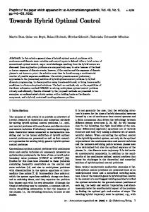
In [15] investigations with unit-disc-graphs and a simplified second order dynamic formulation were done to determine resulting constraints for the continuous control variables. A detailed graph theoretic and an algebraic formulation for modeling k-hop-connectivity constraints are shown in [16]. Also, a centralized framework to control the structure of dynamic graphs has been proposed. On the one hand nonlinear, discrete-continuous N P-hard optimal control problems with heterogeneous conditions have been considered which require for a numerical solution estimations or bounds that are hardly available from theory. Only relatively small problems can be solved under strong assumptions numerically within reasonable computing times. On the other hand there are many heuristic based approaches to control only very specific scenarios of cooperating multivehicle systems. With the work proposed in this paper we aim at bridging this gap between theoretical and practical views. Our approach is founded on the long-term objective to build up an optimization-based model predictive controller (MPC) that considers essential characteristics of cooperative systems and will be applicable to a wide range of scenarios. Therefore we are introducing a general formulation for optimal control of cooperative communicating multi-vehicle systems in structured environments (Sect. II) and are investigating it from the view of hybrid optimal control (Sect. III). Sect. IV focuses on methods to transform the problem into (in-)equalities that can be treated by numerical (non-)linear optimization methods. A representative benchmark problem is proposed and investigated in Sect. V. II. M ATHEMATICAL M ODELING OF C OOPERATIVE M ULTI -V EHICLE S YSTEMS WITH C ONNECTIVITY F EATURES We consider a set of nv cooperating vehicles in a structured environment containing heterogeneous areas with obstacles and different physical environments (e.g. water, air, solid ground, etc.) in R3 . According to the dynamic abilities and according to the environmental constraints we want to determine the optimal vehicle controls for collision-free trajectories in monitoring applications. Therefore we require that a set of areas or waypoints must be traversed or visited by at least one vehicle during the mission. Uninterrupted communication between the moving vehicles is required during operation. A. Modeling of the Environment To cope with realistic outdoor scenarios we are regarding a two dimensional area R ⊂ R2 (cf. Fig. 1 for an example) which is separated into a set of convex subregions, i.e. R=

nR [

Rl .

(1)

l=1

A discrete parameter ql ∈ Q is assigned to each subregion Rl and represents its discrete state relevant to the vehicle’s locomotion. For instance we are distinguishing the states {solid floor, water, building} and use ql ∈ Q = {1, 2, 3} in the system description. The feasible sequences

y 111111 000000 000000 111111 000000 111111 000000 111111 water 000000 111111 000000 111111 000000 R4 R111111 R2 R5 3 000000 111111 000000 111111 000000 111111 000000 111111 000000 111111 000000 111111 000000 111111 000000 111111 solid floor 000000 111111 000000 111111 000000 111111 000000 111111 000000 111111 000000 111111 000000 111111 000000 R9 R8 111111 R7 R10 000000 111111 000000 111111 building 000000 111111 000000 111111 000000 111111 000000 111111 R13111111 000000 R15 R14 R12 00 11 000000 111111 00 11 000000 111111 00 11 start / finish xObst,1 xObst,2

R1 0 1 0 1 0 1

R6 R11

yObst,1

yObst,2 x

Fig. 1. Partitions of a considered area with a building (R7 ) and a river (R4 ∪ R9 ∪ R14 ) which are denoted by dashed lines. R1 q1

R2 q1

R6 q1 R11 q1

Fig. 2.

R12 q1

R3 q1

R5 q1

R8 q1

R10 q1

R13 q1

R15 q1

Graph of connected feasible regions for a ground vehicle in Fig. 1.

of regions where a single vehicle can locomote through is described by a (not necessarily) connected graph Gvi = (Vvi , Evi )

(2)

with Vvi ⊂ {Rl | l = 1, ... nR } and Evi ⊂ Vvi × Vvi . E.g. the graph in Fig. 2 results for a ground vehicle and the environment of Fig. 1. Each subregion Rl is described by its boundaries, "Ã ! # £ ¤ xvi ∈ Rl ⇔ g Rl (xvi , yvi ) ≤ 0 , (3) yvi where (xvi , yvi )T is the (vehicle’s) position in the twodimensional case with a suitable vector function g Rl . Here “≤” denotes the component wise comparison of two vectors. B. Locomotion Properties of a Single Vehicle Various types of vehicles are considered (cf. Fig. 1). It is assumed that the motion dynamics of each vehicle vi in a certain physical environment (described by the discrete state ql which is used as an index) can be modeled by a system of (usually nonlinear) first order ordinary differential equations x˙ vi (t) = f vqli (xvi (t), uvi (t)) .

(4)

The trajectory xvi (t) ∈ Rnx,vi represents the continuous state variables (including position, velocity and orientation) and uvi (t) ∈ Rnu,vi the continuous control variables (e.g. accelerating and braking forces). Depending on the level of physical detail, these equations of motion range from approximative linear to complex, nonlinear dynamic equations. The dimensions of xvi and uvi also vary according to the vehicle’s type of locomotion (walking, driving, swimming, flying etc.). The state xvi (0) = xv0i of the vehicle at the initial time t0 = 0

is assumed to be known (or may be optimized as well). The state and control variables are constrainted at each time t by ∃1 l ∈ {1, ... , nR } : £ ¤ V vi vi g Rl (xvi (t)) ≤ 0 g ql (x (t), uvi (t)) ≤ 0 ,

(5)

where g vqli denotes physical constraints of the specific vehicle, e.g., on its maximum velocity or acceleration. The set of feasible indices ql ∈ Q is determined by the different vehiclespecific modes of locomotion according to the discrete states characterizing the subregions. Constraints according to the boundaries of the subregions Rl in which the vehicle is currently moving are expressed by g Rl (cf. Eq. (3)). The respective logical conditions in Eq. (5) can be transformed into a set of linear inequalities eventually. For crossing the regions’ borders a fixed number of switching times (which may be given or free) t0 = ts,0 < ts,1 < ... < ts,k < ... < ts,ns = tf ts,k − ts,k−1 < tmin (k = 1, . . . , ns )

(6) (7)

is introduced. The discrete states Rl (and ql resp.) can change their values only at one of these timepoints. Feasible sequences i i (g vql,1 , ..., g vql,n ) of active constraints for a fixed number ns of s possible switching times are defined implicitly in Sect. II-A. The constant tmin in Eq. (7) is motivated by the minimal time span that is needed to perform the desired tasks, e.g. collecting data in a subregion in the case of monitoring missions. It is also required that the variables xvi and uvi are continuous xvi (ts,k − 0) = xvi (ts,k + 0), uvi (ts,k − 0) = uvi (ts,k + 0),

(8)

at switching time ts,k with t ± 0 := lim²→0,²>0 t ± ². To introduce communication in this motion model we have to think of transmitting and of receiving information. Receiving mainly depends on the strength of available signals. For (wireless) broadcasting of information a detailed wave propagation model would be needed. For the purpose of cooperative optimal vehicle trajectories, we will consider communication by approximating connectivity functions (Sect. II-D). The problem of computing the optimal control for a single vehicle subject to the constraints (4) - (5) has been well investigated with various methods. Now the question of optimal controls for a cooperative multi-vehicle system under the requirement of connectivity is posed. C. Requirements of Multiple Cooperating Vehicles To cope with multiple vehicles the model is augmented by collision avoidance constraints i ∀vi 6= vj , ∀t : g vcoll (xvj (t), yvj (t)) ≤ 0 ,

(9)

where (xvj , yvj )T denotes the position of vj . Also a task (or a set of sub-tasks) is needed for the multi-vehicle cooperation. In the context of monitoring scenarios we require that a certain

part R∗l ⊂ Rl of each region Rl must be investigated by at least one vehicle at least one time during the mission à ! xvi (t) ∀Rl ∃ t ∈ [t0 , tf ] ∃ i ∈ {1, ...nv } : ∈ R∗l . (10) yvi (t) D. Connectivity and Network Topology The ability of sharing information is assured by the permanent existence of a stable connectivity network. This includes constraints on the network topology, on the network’s alteration in time and on the rigidity of the radio link itself. For each vehicle we consider a function Cvi that describes the radiowave propagation of object vi depending on its position and the point (x, y, z)T where we are interested in the signal strength. Thus, for a pair (vi , vj ) of vehicles and for a required signal strength cvj of vehicle vj we define a binary variable a ˜vi ,vj ∈ {0, 1} according to       xvi (t) xvj (t) £ ¤       a ˜vi ,vj (t) = 1 ⇔ Cvi ( yvi (t)  ,  yvj (t) ) ≥ cvj  (11) zvi (t) zvj (t) where (xvi , yvi , zvi )T denotes the position of vehicle vi at time t. The motivation of the usually continuous function Cvi ranges from simple distance assumptions in a free-space propagation model until detailed ray tracing models including reflections, slow-fading and fast-fading effects. Stochastic models are also very popular in this context. ˜ The quadratic matrix function A(t) = (˜ avi ,vj (t)) ∈ nv ×nv {0, 1} now describes all possible transmissions in the system from object vi to object vj iff a ˜vi ,vj = 1. In most applications with a high level of cooperation a twoway communication is desired and thus symmetric matrices A = AT are considered. Therefore we set       xvi (t) xvj (t)       Cvi ( yvi (t)  ,  yvj (t) ) ≥ cvj       £ ¤  zvi (t)  zvj (t)  avi ,vj = 1 ⇔    xvj (t) xvi (t)  V        Cvj ( yvj (t)  ,  yvi (t) ) ≥ cvi   zvj (t) zvi (t) (12) The symmetric matrix A(t) = (avi ,vj ){1,...nv }2 now defines the adjacency matrix for the communication network topology ½ 1 if vehicles j1 and j2 are connected, (13) aj1 j2 (t) := 0 otherwise. With ∀t ∈ [t0 , tf ) : A(t) ∈ C we consider that A is part of a finite set of feasible network topologies C. The set of elements in C can be defined with logical expressions or algebraic constraints itself. E.g for fault tolerance, δconnectivity is desirable. For quality of service investigations k-hop connectivity is considered (cf. [16]). To obtain a suitable topology control we require that changes in the network structure can only occur at discrete switching times, which were defined in Eq. (6). In this context Ak := A(t), ts,k−1 ≤ t ≤ ts,k , i = 1, . . . , ns ,

(14)

is defined. The constraint of Eq. (7) guarantees some stability in the topology. If there is a significant difference between the time for fulfilling the task and the time which is required for a constant network topology, then Eq. (7) has to be replaced by a more detailed structure in the switching times. Possibly additional logical expressions are needed therefore.

with constant lower and upper bounds. In general not all discrete states ρk can follow or proceed each other. Thus, additional logical constraints must be considered: © ¡ ¢ª true l ρ1 , . . . , ρns . (21)

III. A H YBRID O PTIMAL C ONTROL A PPROACH The evolution in time of the discrete states (i.e., network topology, mode of locomotion according to the environment) and the resulting continuous vehicle trajectories of the problems considered are tightly coupled. Thus the problem of computing the best solution is characterized by its combinatorial part and its relation to the (nonlinear) dynamic optimization part. We now propose a general description for the general problem as nonlinear hybrid optimal control problem. For this purpose, we consider a feasible sequence of ns discrete system states ρk ,   Rl   ρ(t) :=  q(t)  ∈ Vv1 × ... × Vvnv × Qnv × C (15) A(t) ρk := ρ(t), ts,k−1 ≤ t ≤ ts,k , i = 1, . . . , ns . Pnv nx,vi ) and also If the initial state x(0) ∈ Rnx (nx = P i=1 nv nu,vi ) are given the control history u(t) ∈ Rnu (nu = i=1 then state trajectory x(t) can under mild assumptions uniquely be determined from integration of

We now discuss the general formulation of the objective function (17) to be minimized and give some common cases. The first part ϕns (x(tf ), tf ) is responsible for all effects at the final time. This part contains desired final states or regions, if the final time is fixed. If the final time is free, tf itself may appear in ϕns . With ϕk (x(ts,k − 0), x(ts,k + 0)) the costs for state transitions are measured. Here, switches in the communication network topology or changes in the environmental conditions for locomotion are considered. The function Lk (x(t), u(t), t) represents other physical values depending on the vehicles’ motions, e.g. energy consumption. Some most common examples are explained in the following which may also be used in combination as a weighted sum. 1) Minimizing the Energy: Especially to cope with aerial vehicles it often is important to plan a mission with minimal energy consumption to reduce the vehicles’ battery packs or extend their time of operation. A typical formulation is ns Z ts,k X J= (u(t))T (u(t))d t . (22)

˙ x(t) = f ρk (x(t), u(t), t), ts,k−1 < t < ts,k ,

(16)

k = 1, . . . , ns , 0 ≤ t ≤ tf . We assume all x(t) and u(t) to be continuous at the switching times ts , although it is possible to consider also jump or switching conditions. A HOCP is considered where we wish to determine the optimal sequence of actions of the cooperating vehicles, i.e. the discrete state values ρk , k = 1, . . . , ns . Here, ns as well as the continuous control history u(t), 0 ≤ t ≤ tf , and the switching times ts,1 , . . . , ts,ns = tf are to be determined in a way that the cost function

A. Objective Function

k=1

ts,k−1

2) Minimizing the Final Time: If we are interested in the shortest, possible time to complete the mission, a possible form of the objective function (17) reads as ns Z ts,k X J = tf + ε (u(t))T (u(t)) d t (23) k=1

ts,k−1

with ε = 0. However, with a small ε > 0 the second addend ensures the uniqueness and some regularity of the solution because otherwise only a fast trajectory for the slowest vehicle would be computed but the resulting trajectories of the other vehicles would in general not be uniquely determined then. 3) Stabilizing Connectivity and Network Topology: Desired network properties like bi-connection stability results can min J, (17) u,ρ1 ,...,ρns be formulated. For instance the values of the connectivity Pns −1 functions cvi (cf. Eq. (12)) can be considered for optimization J = ϕns (x(tf ), tf ) + k=1 ϕk (x(ts,k − 0), x(ts,k + 0)) Pns −1 Pns R ts,k J= + L (x(t), u(t), t) d t k=1 ϕk (x(ts,k − 0), x(ts,k + 0)) k k=1 ts,k−1 Pnv Pns R ts,k c (x(t)) d t (24) − i=1 c˜i · k=1 ts,k−1 vi with real-valued functions ϕk , Lk is minimized subject to the equations of motion (16), the initial condition x(0) = x0 , with suitable constants c˜i . constraints on the final state IV. N UMERICAL T REATMENT 0 = r eq,ρns (x(tf )) , 0 ≤ r iq,ρns (x(tf )) , (18) A. Hybrid Nonlinear Optimal Control and constraints on the (continuous) state and control variables If a maximum number of switching times (i.e. transitions in (ts,k−1 , ts,k ], k = 1, . . . , ns , in network topologies or soil conditions) is assumed, then an 0 ≤ g ρk (x(t), u(t), t), uρk ,min xρk ,min

≤ u(t) ≤ ≤

x(t)

≤

uρk ,max , xρk ,max

(19) (20)

unknown sequence of discrete state variables ρk (Eq. 15) can be transformed into a sequence of integer variables ρ∗k ∈ I ⊂ Nns which can be represented by a vector of binary variables b ∈ {0, 1}nb . The feasibility of succeeding or

1. phase 2. phase x˙ = f q 1 (.)

x(0)q

0 = ts,0

ts,1

i. phase x(t) x˙ = f q (.)

ts,2 ts,i−1

i

ts,i

B. Linear Mixed-Binary Optimal Control Problem Approximation qx(tf ) ts,ns = tf

t

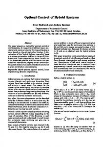
Fig. 3. Illustration of a continuous state trajectory x(t) with nonlinear state dynamics defined in ns phases. Phase transitions occur at switching times ts,k .

preceding actions, phases or nodes is described by constraints as in Eq. (21). Thus, the previously introduced hybrid optimal control problem is transformed into a mixed-integer, namely mixed-binary, dynamic optimization problems (MBOCP) and numerical methods for this class of problems can be applied. The numerical solution approach consists of a decomposition of MBOCP in coupled discrete and dynamic optimization problems (cf. [17], [18] for details). In an inner loop the continuous dynamic part of the optimization problem is considered according to its constraints (Eqs. (16), (19)) for the fixed number of ns phases (Fig. 3). For each phase [ts,k−1 , ts,k ] a time discretization grid is introduced. Along this time grid the continuous state variables x(t) and the control variables u(t) are approximated by piecewise polynomial functions [18]. Thus, the dynamic optimization problem is transformed into a large, sparse nonlinear constrained optimization problem which is solved numerically by a sparse sequential quadratic programming method [19]. At the outer iteration level an investigation of the discrete solution space is performed. For this purpose, Branch-and-Bound (B&B) methods are applied. Their performance depends on the way estimates of good lower and upper bounds on the cost function (17) are obtained and maintained (cf. [18]). These non-convex mixed-integer optimal control problems require efficient numerical methods to cope with their combinatorial characteristics. Bounds and solution estimates for the full, nonlinear problem are key stages towards efficient computation of optimal controls in cooperative systems. Fast computable, global bounds could be used to exclude many unprofitable sequences of states, but are hardly available. The combinatorial part makes it difficult to find good, proven global bounds and the high dimensions of the resulting nonlinearly constrained optimization problems (NLPs) in the inner loop complicate a fast numerical computation of them. Therefore, we investigate a transformation of the HOCP to MILPs to enable reasonably fast computation of solution estimates as motivated by results from [3], [4]. The MILPs must account for the significant structure of the original problem and can be solved efficiently with available software. The MILP solutions may later serve either as initial estimates for the numerical HOCP solution or for intermediate steps in a model predictive approach.

We are now describing the general formulation for the mixed-integer linear model. Our intention is to transform the whole cooperative optimal control problem into the form à ! à ! à ! x ˜ x ˜ x ˜ ˜1 ˜2 min cT s.t. A =˜ b1 , A ≤˜ b2 (25) u ˜ u ˜ u ˜ ˜1 , A ˜2 and vectors ˜ with real-valued matrices A b1 , ˜ b2 , c. Here, n1 n3 x ˜ ∈ R × {0, 1} denotes the state variables and u ˜ ∈ Rn2 × {0, 1}n4 control variables (nA := n1 + n2 + n3 + n4 ). There have been shown many advantages of these linear models. Particularly their robustness and efficiency without requiring good initial solution estimates made them applicable to many online control algorithms in cooperative scenarios. The most restrictive modification in our transformation of the original nonlinear optimal control problem results from the introduction of a fixed (not necessarily equidistant) time grid T (resp. sampling time T s ) T

:=

(t1 , ..., tk , ...tN +1 )T

Ts

:=

(t2 − t1 , ..., tk+1 − tk , ...tN +1 − tN )T

=:

(t1 , ..., tk , ...tN )T .

(s)

(s)

(26)

(s)

Thus the switching times of Eq. (15) have to coincide with elements from T and are not freely adjustable any more. With x(k) and u(k) we denote the vectors whose elements are associated with the time step tk+1 . Assuming that a feasible control variable u(k) is given, the evolution of the system à ! x(k) (27) x(k + 1) = Ak u(k) is then fully determined by initial and/or final conditions x(1) = x0 , x(N + 1) = xf . The transformation of Eq. (16) into the linear approximation of Eq. (27) has to be done with caution to account for the characteristics of a specific fρk . It may be necessary to distinguish different cases and to introduce additional variables. Jump and switching conditions are modeled as X x(k + 1) = x(k) + bρi ,ρj (k) γ ij , (28) i,j

with a vector of constants γ ij . The binary variable bρi ,ρj equals 1 iff the system switches from state ρi to ρj . Inequalities are transformed analogously. The constraints on control and state variables (19) result in a set of binary variables bρi and linear expressions à ! x Hρk + bρk · γρk ,1 ≤ γρk ,2 . (29) u The constant values in γρk ,1 and γρk ,2 can partly be determined by using the “Big-M”-technique (cf. [20]). Some cases of these constraints are proposed in Sect. V.

vehicle ground vehicle

number j 1

wjU B 15

B uU j 1.5

ground vehicle

2

15

1.5

ship aerial vehicle

3 4

10 30

0.8 3

allowed zones Rl 1, 2, 3, 5, 6, 8, 10, 11, 12, 13, 15 1, 2, 3, 5, 6, 8, 10, 11, 12, 13, 15 4, 9, 14 1, 2, ..., 15

TABLE I T HE VEHICLES ’ PARAMETER

As already noted, the number of different cases highly increases in modelling with only linear expressions. Thus in addition to Eq. (21) logical constraints are needed. They result in a system of linear expressions L b ≤ γL where b represents all introduced binary variables. To investigate the potential of the proposed combined method, we propose and investigate a representative example of a mixed-integer linear model. First promising results are reported in Sect. V-B. V. R EPRESENTATIVE E XAMPLE Optimal control of the multi-vehicle system in the following scenario is investigated: Given are nv = 4 vehicles in the environment of Fig. 1 and a final time tf . What are the energy-minimal trajectories for the vehicles subject to the requirements that a certain part R∗l of each region Rl must be visited at least once, that the vehicles do not collide and that connectivity is guaranteed anytime? The complexity of distributing the selection and sequence of nR zones of interest R∗1 . . . R∗15 in a plane area (Fig. 1) to be visited by at least one of the cooperating individual vehicles together with determining optimal vehicle motion trajectories arises with the combinatorial character in the switched constraints. Therefore we start with a simple point mass model for vehicle vj in R2 . The approach presented in this paper also allows a spatial as well as more general settings. The vehicles (or mass points respectively) are starting at the origin at initial time t0 = 0 and are ending at the origin at the final time tf . Thus the model reads as x˙ j (t) = wx,j (t), y˙ j (t) = wy,j (t), w˙ x,j (t) = ux,j (t), w˙ y,j (t) = uy,j (t), 2 2 wx,j + wy,j ≤ (wjU B )2 ,

xj (0) = 0 = xj (tf ), yj (0) = 0 = yj (tf ), wx,j (0) = 0 = wx,j (tf ), (30) wy,j (0) = 0 = wy,j (tf ), B 2 u2x,j + u2y,j ≤ (uU j ) T

.

Hereby xj = (xj , yj , wx,j , wy,j ) where xj , yj denote the position, wx,j , wy,j the corresponding velocities and uj = T (ux,j , uy,j ) the acceleration or brake forces of the vehicle which are constrained. According to the different dynamic motion abilities, we are considering the bounds given in Table I. Requiring the vehicles’ position in the zones of interest for each R∗l the boundary condition reads as "Ã ! # nv _ ns _ xj (tk ) ∗ ∈ Rl . (31) yj (tk ) j=1 k=1

The zones of interest R∗l are defined according to the borders of Rl and a distance dR∗ ∈ R such that ! à ! à ∗ x ± d x R ∈ R∗l ⇒ ∈ Rl . (32) y y ± dR∗ Using the binary values bkj,l ∈ {0, 1} (k = 1, . . . , ns , j = 1, . . . , nv , l = 1, . . . , nR ) the statement bkj,l = 1 → (x, y)T ∈ R∗l can be expressed by à ! xj (tk ) Hl − Γl + bkj,l M l ≤ M l . (33) yj (tk ) The rows of matrix H l contain all coefficients of the linear borders of the according zones, i.e. each representative row of Eq. (33) for zone Rl looks like αl x + βl y − γl + bij,l · Ml ≤ Ml . Γl and M l are vectors of constant values such that à ! xj (tk ) M l ≤ max(H l − Γl ) . yj (tk )

(34)

(35)

To guarantee that each zone is visited by a vehicle at least once during the mission we require     nR X ns X nv ns X nv ^ X X ∀l : bkj,l = 1 . (36) bkj,l = 1  l=1 k=1 j=1

k=1 j=1

For collision-free trajectories between a pair (j1 , j2 ) of vehicles we additionally require ¯¯Ã !¯¯ ¯¯ x (t) − x (t) ¯¯ j2 ¯¯ j1 ¯¯ ∀i1 6= i2 , ∀t0 ≤ t ≤ tf : ¯¯ ¯¯ ≥ rmin . (37) ¯¯ yj1 (t) − yj2 (t) ¯¯ 2

In our example we consider this collision constraint for the ground vehicles (j1 , j2 ) = (1, 2) and outside a start/finishzone around (0, 0). The whole area of Fig. 1 is described by |xj (t)| ≤ yj (t) ≤

400, yj (t) ≥ 600, yj (t) − xj (t) ≥

0, 440.

(38)

Table I shows the feasible regions where each vehicle is allowed to move. All other regions have to be treated as obstacles. Therefore we require for the ground vehicles j ∈ {1, 2} "Ã ! # ^ ^ xj (t) ∈ / Rl . (39) yj (t) j∈{1, 2} l∈{4, 7, 9, 14}

Obviously in the instance of the quadratic obstacle (i.e. the building) R7 we can also require ¬ [(xj ≥ xObst,1 ) ∨ (xj ≤ xObst,2 )∨ (yj ≥ yObst,1 ) ∨ (yj ≤ yObst,2 )]

(40)

for j ∈ {1, 2}. xObst and yObst are the borders of the obstacle as defined in Fig. 1. The constraints for the ship (j = 3) and the aerial vehicle (j = 4) are formulated respectively.

For the purpose of demonstration we consider a simple two dimensional connectivity function for each vehicle j q −1 cj ((xj , yj )T ,(x, y)T ) = (xj − x)2 + (yj − y)2 + 2 130 (41) " # cj1 > 1 V ⇔ [akj1 ,j2 = 1] . (42) cj2 > 1 We require vehicles to be connected for each time step k by nv nv X X

akj1 ,j2 ≤ 1 .

(43)

j1 =1 j2 >j1

A. Linearized Implementation We are now showing a completely linearized implementation of the introduced example by applying the formalism of Sect. IV-B. For the purpose of demonstration equidistant fixed time steps ts are used. Thus the motion dynamics (30) is transformed to xj (k + 1) = wx,j (k + 1) =

xj (k) + ts wx,j (k) wx,j (k) + ts ux,j (k) ,

(44) (45)

(yj , wy,j , analogously), where wx,j denotes the velocity of vehicle j in the direction of x. Initial and final conditions are given by (yj and wy,j respectively)

For the considered ground vehicles (j ∈ {1, 2}) the zone R7 is regarded as an obstacle [xObst,1 , xObst,2 ] × [yObst,1 , yObst,2 ]. Therefore we transform (40) into −xj (k) − b1O MO,x xj (k) − b2O MO,x −yj (k) − b3O MO,y −yj (k) − b4O MO,y

≤ ≤ ≤ ≤

−xObst,2 xObst,1 −yObst,2 yObst,1

(51)

2 ≤ b1O + b2O + b3O + b4O ≤ 4 with binary variables bO and a constants MO,x ≥ max{−xj (k) + xObst,2 , xj (k) − xObst,1 } (MO,y resp.). In our example we are using xObst,1 = −240, xObst,2 = −80 and yObst,1 = 80, yObst,2 = 240. To improve our model we are additionally requiring xj (k) + xj (k + 1) − bv (2 · (xObst,2 ) + MT ) > −MT yj (k) + yj (k + 1) + bv · MT < 2(yObst,1 ) + MT

(52) (53)

with MT ≥ 2 · maxk {xk , yk }(const.) to avoid tunneling under the vertices (−80, 80) of obstacle R7 . All other vertices are treated respectively. According to Table I all other infeasible zones have to be implemented for each vehicle analogously. For collision avoidance between the vehicles we are using simple box constraints following the ideas in Eq. (48) with nγ = 4 and r = 18. To model the connectivity we transformed Eqs. (41) and (42) into

(46) (47)

i i sin( π)(xj1 (k) − xj2 (k)) + cos( π)(yj1 (k) − yj2 (k)) 3 3 + bck,j1 ,j2 Mc ≤ 130 + Mc (54)

In the investigated example the controls and velocities are constraint bypquadratic expressions. In general expressions of the form ± (x1 − x2 )2 + (y1 − y2 )2 ≤ ±r can be transformed by using a set of nγ ≥ 4 linear expressions

where Mc ≥ max{|xj1 − xj2 |, |yj1 − yj2 |}, i = 1, . . . , 4, and j1 = 1, . . . , nv , j1 < j2 . Thus together with Eq. (43) the connectivity between the vehicles is modeled.

−3 ≤ xj (1) ≤ 3 ; xj (N + 1) = 0 wx,j (1) = 0 = wx,j (N + 1) .

i i ± sin( π) (x1 − x2 ) ± cos( π) (y1 − y2 ) ≤ ±r , 3 3

(48)

i = 1, . . . , nγ . Thus the bounds on the controls (30) become 8 ^ £ ¤ B ≤0 sin( 3i π) ux,j + cos( 3i π) uy,j − uU j

(49)

i=1

in our implementation. We are also using these polygons to formulate the objective function where we are intending do minimize the energy for our mission. Another variable qu,j is introduced such that 8 ^ £ ¤ sin( 3i π) ux,j + cos( 3i π) uy,j ≤ qu,j

(50)

i=1

Pnv and we are minimizing J = j=1 qu,j . To guarantee that each zone is visited at least once during the mission we are implementing the inequalities (33) and equalities (36).

B. First Numerical Results In a first straight-forward linearized implementation of the proposed benchmark problem we dropped the collision avoidance constraints resulting in a MILP with 1616 variables and 12112 (in-)equality constraints. This MILP was solved using CPLEX [21] and the free Matlab [22] interface CPLEXINT [23] in about 79 min. The computation was started without any initial guesses and without a (certainly very helpful) decoupling which we expect to reduce the computational time of the straight-forward implementation by a factor of about ten. The Figs. 4 and 5 show the approximated trajectories for optimal controls and positions resulting from the MILP-model in direction in x and y. In Figs. 6 and 7 the resulting paths in the x-y-space are shown with the underlying communication network. VI. C ONCLUSIONS AND O UTLOOK A general methodology for modeling and optimizing cooperative multi-vehicle systems that are mainly characterized by their motion dynamics has been proposed. The influence

ground veh.

2

ship

0 −1

500

400

400

300

300

200

200

100

100

0 −1

−2

−2

0

20

40 time

Fig. 4.

60

80

0

20

40 time

60

80

0 −400

Controls ux (left) and uy (right) of the vehicles.

400

100

300

0

200

x

100

−200

0

−300 0

20

Fig. 5.

40 time

60

−100 0

80

20

40 time

60

80

Positions x (left) and y (right) of the vehicles.

of connectivity required for communication on optimal multivehicle trajectories has been considered in the models. The presented approach is in principle not restricted to a certain class of robots or tasks and can be applied to different kinds of multi-vehicle systems. Results have been presented for an optimal cooperative control problem of four heterogeneous vehicles subject to motion dynamics, heterogeneous motion constraints and connectivity constraints for wireless communication. The MILP based approach presented in this paper may be applied for different purposes, e.g., to evaluate the degree of optimality of heuristic, distributed real-time coordination and control schemes or to compute good bounds or initial solution estimates for numerical methods tackling the general HOCP formulation. Also, mixed-integer linear models itself may be developed further towards online application in a modelpredictive control method for multiple vehicles in uncertain environments. Such a method could be based on repeated online solution of MILPs which are properly adapted to cover changes in the world model as it is the the case in many cooperative robot problems like robot games or monitoring and surveillance scenarios.

600

600

500

500

400

400

300

300

200

200

100

100

−300

−200

−100

0

100

200

300

400

0 −400

−300

−200

−100

0

100

200

−300

−200

−100

0

100

200

300

400

0 −400

−300

−200

−100

0

100

200

300

400

Fig. 7. After the timesteps t12 = 83.1 (left) and t14 = 96.9 (right): The second ground vehicle did not yet leave the starting position but stays connected to the others. The aerial vehicle flies across the river and holds connection to the ship ( ).

y

200

−100

0 −400

600

500

1

aerial veh. uy

u

x

1

600

2

ground veh.

300

400

Fig. 6. After the first timesteps t6 = 41.5 (left) and t8 = 55.4 (right): ) moves around the building where the aerial One of the ground vehicles ( vehicle ( ) flies over it. ( ) shows the communication network.

ACKNOWLEDGMENT The authors thank Alexander Martin, TU Darmstadt, for helpful discussions about MILP and for software support as well as Matthias Kropff and Matthias Hollick, TU Darmstadt, for helpful discussions about communication networks. Parts of this research have been supported by the German Research Foundation (DFG) within the Research Training Group 1362 “Cooperative, adaptive and responsive monitoring in mixed mode environments”. R EFERENCES [1] A. Richards, J. Bellingham, M. Tillerson, and J. How, “Coordination and control of multiple UAVs,” in Proc. AIAA Guidance, Navigation, and Control Conf., Monterey, CA, 2002. [2] J. Gancet, G. Hattenberger, R. Alami, and S. Lacroix, “Task planning and control for a multi-UAV system: architecture and algorithms,” in IEEE Intl. Conf. on Intelligent Robots and Systems, Edmonton, CAN, 2005. [3] A. Richards and J. P. How, “Aircraft trajectory planning with collision avoidance using mixed integer linear programming,” in ACC. IEEE, May 2002, pp. 1936 – 1941. [4] M. Earl and R. D’Andrea, “Iterative milp methods for vehicle control problems,” IEEE Transactions on Robotics, vol. 21, no. 6, pp. 1158– 1167, December 2005. [5] F. Borrelli, D. Subramanian, A. Raghunathan, and L. Biegler, “MILP and NLP techniques for centralized trajectory planning of multiple unmanned air vehicles,” in American Control Conference, 2006. [6] T. Furukawa, F. Bourgault, H. F. Durrant-Whyte, and G. Dissanayake, “Dynamic allocation and control of coordinated UAVs to engage multiple targets in a time-optimal manner,” IEEE Intl. Conf. on Robotics & Automation, pp. 2353–2358, 2004. [7] M. Glocker, C. Reinl, and O. von Stryk, “Optimal task allocation and dynamic trajectory planning for multi-vehicle systems using nonlinear hybrid optimal control,” in Proc. 1st IFAC-Symposium on Multivehicle Systems, Salvador, Brazil, October 2-3 2006, pp. 38–43. [8] M. Glocker and O. von Stryk, “Hybrid optimal control of motorized traveling salesmen and beyond,” in Proc. 15th IFAC World Congress on Automatic Control. Barcelona, Spain: Elsevier Science, July 21-26 2002, pp. 987–992. [9] F. M. Landstorfer, “Wave propagation models for the planning of mobile communication networks,” European Microwave Week 1999, Munich (Germany), (Invited Paper), 1999. [10] F. Xue and P. Kumar, “The number of neighbors needed for connectivity of wireless networks,” Wireless Networks, vol. 10, no. 2, pp. 169–181, 2004. [11] D. Blough, M. Leoncini, G. Resta, and P. Santi, “The k-neigh protocol for symmetric topology control in ad hoc networks,” in Proc. 4th ACM Intl. Symposium on Mobile Ad Hoc Networking and Computing (MobiHoc’03), 2003, pp. 141–152. [12] N. Li and J. C. Hou, “Topology control in heterogeneous wireless networks: problems and solutions,” in Proc. IEEE INFOCOM, 2004. [13] D. Spanos and R. Murray, “Robust connectivity of networked vehicles,” in 43rd IEEE Conference on Decision and Control, 2004. CDC, vol. 3, 2004, pp. 2893– 2898.

[14] P. Basu and J. Redi, “Movement control algorithms for realization of fault-tolerant ad hoc robot networks.” IEEE Network, vol. 18, no. 4, pp. 36–44, 2004. [15] G. Notarstefano, K. Salva, F. Bullo, and A. Jadbabaie, “Maintaining limited-range connectivity among second-order agents,” in American Control Conference, Minneapolis, MN, USA, 2006. [16] M. M. Zavlanos and G. J. Pappas, “Controlling connectivity of dynamic graphs,” in 44th IEEE Conf. on Decision and Control, Sevilla, Spain, 2005, pp. 6388–6393. [17] M. Buss, M. Glocker, M. Hardt, O. von Stryk, R. Bulirsch, and G. Schmidt, “Nonlinear hybrid dynamical systems: modeling, optimal control, and applications,” in Modelling, Analysis and Design of Hybrid Systems, ser. Lecture Notes in Control and Information Sciences, E. S. S. Engell, G. Frehse, Ed., vol. 279. Berlin, Heidelberg: Springer-Verlag, 2002, pp. 311–335. [18] O. von Stryk and M. Glocker, “Numerical mixed-integer optimal control and motorized traveling salesmen problems,” APII-JESA (Journal europ´een des syst`emes automatis´es - European Journal of Control), vol. 35, no. 4, pp. 519–533, 2001. [19] P. Gill, W. Murray, and M. Saunders, “SNOPT: An SQP algorithm for large-scale constrained optimization,” SIAM J. Optim., vol. 12, pp. 979– 1006, 2002. [20] A. Bemporad and M. Morari, “Control of systems integrating logic, dynamics, and constraints,” Automatica, vol. 35, no. 3, pp. 407–427, 1999. [21] ILOG CPLEX 10.0, User’s Manual, ILOG, Inc., 2006. [22] Matlab 7.3, TheMathWorks, http://www.mathworks.com. [23] F. Torrisi and M. Baotic, CPLEXINT - Matlab interface for the CPLEX solver, http://control.ee.ethz.ch/˜hybrid/cplexint.php.