Optimal Filtering and Smoothing for Speech Recognition ... - CiteSeerX

Optimal Filtering and Smoothing for Speech Recognition Using a Stochastic Target Model G. Ramsay and L. Deng

Department of Electrical & Computer Engineering University of Waterloo Waterloo, Ontario, Canada N2L 3G1.

ABSTRACT This paper presents a stochastic target model of speech production, where articulator motion in the vocal tract is represented by the state of a Markov-modulated linear dynamical system, driven by a piecewise-deterministic control trajectory, and observed through a non-linear function representing the articulatory-acoustic mapping. Optimal ltering and smoothing algorithms for estimating the hidden states of the model from acoustic measurements are derived using a measure-change technique, and require solution of recursive integral equations. A sub-optimal approximation is developed, and illustrated using examples taken from real speech.

1. Introduction The modelling of temporal and contextual variation observed in the acoustic signal is a central concern in speech recognition, and is not handled well by traditional HMM methodologies. Since much of the observed variability in speech can be attributed to articulatory dynamics, it is reasonable to assume that incorporation of an explicit model of articulatory phenomena should eventually lead to improved performance, and to a more compact and precise parameterization of many sources of contextual variation. In a recent paper [1], we proposed a stochastic target model of speech production, where articulator motion in the vocal tract is represented by the state of a linear dynamical system observed through a non-linear function representing the articulatory-acoustic mapping. The system parameters are modulated by a Markov chain representing phonological sequences, and the system is driven by a control input consisting of a piecewise-deterministic trajectory modelling dynamic targets in the articulatory space. The contribution of the present paper is the derivation of the optimal non-linear ltering and smoothing recursions needed to estimate the hidden states of the model from acoustic measurements. Results from a full articulatory recognition task are not yet available, but data- tting experiments on cepstral data from real speech are provided to illustrate a number of phenomena aecting performance.

2. Model Formulation

Assume an underlying complete probability space ( ; F ; P ). Let S = fSm : m 2 INg be a nite-state homogeneous Markov chain generating phonological sequences, taking values in a nite alphabet S = fsi : i = 1 : : : NS g. De ne a transition matrix  = [(i; j ) : i; j 2 S ], where (i; j ) = P (Sm+1 = j jSm = i), (i; j )  0, j2S (i; j ) = 1, and assign an initial distribution 1 : S ! [0; 1].

P

Let T = fTm : m 2 INg be a process representing the durations of the states in S , where each Tm is drawn from a Poisson distribution with mean  (Sm ) chosen from a family of duration parameters T = f (i) 2 IR : i 2 Sg De ne also  = fm : m 2 INg, where 1 = 1, m = m 1 + Tm (8m > 0). To simplify notation, construct a Markovian representation Z = fZn : n 2 INg of the semi-Markov chain (S; T ), where Zn takes values in a countable state-space Z = fzti : i 2 S ; t 2 INi g and de nei mappings fS : Z ! S , fT : Z ! IN by fS (zt ) = i, fT (zt ) = t. Let  and 1 be the transition matrix and initial distribution for Z such that the processes (fS (Zm ); fT (Zm+1 1 )) and (Sm ; Tm ) are indistinguishable. Each phonological sequence produced by (S; T ) induces a statistical distribution of possible target trajectories on an articulatory space X = IRp , representing abstract motor commands. The trajectories are assumed to be piecewisedeterministic, in that the shape of any section of trajectory corresponding to a particular state is de ned by parameters drawn from an associated probability distribution when the state is entered. The subsequent evolution of the trajectory is completely determined by these parameters until the next phonological transition occurs. The shape of each parameter distribution models systematic static/dynamic compensatory eects in realizing a particular phonological unit. A previous paper presented a model for piecewise-constant trajectories, where the distributions modelled variation in absolute spatial targets. Here we present an extension that allows for piecewise-polynomial trajectories, where distributions describe the oset (position), slope (velocity), etc., with optional continuity constraints across segment boundaries.

Let U = fUn : n 2 INg be a process representing target trajectories in X . Assume that the sample paths of U consist of polynomial segments U[m ;m+1 ) of order Q, with coecients drawn from a family of distributions = f (i; j ) : i 2 S ; j = 1 : : : Qg according to the current Markov state Sm . Suppose for convenience that (i; j )  N (u (i; j ) 2 IRp ; u (i; j ) 2 IRpp ), de ned by a set of target parameters U = f(u (i; j ); u (i; j )) : i 2 S ; j = 1 : : : Qg. To obtain a Markovian representation for U , de ne processes U i = fUni : n 2 INg : i = 0 : : : Q, i = f in : n 2 INg : i = 1 : : : Q, such that U i records the i'th dierence of the target process U  U 0 , and i records changes in the i'th polynomial coecient. These are generated by the recursion in = Uni =

1 1 IBi (Zn )[u (fS (Zn ); i) + u2 (fS (Zn ); i)Vni ] + 
2 Vni ; IAci (Zn )[Uni 1 + Uni+11 ] + in+1 ;

where V i = fVni : n 2 INg are zero-mean, unit variance Gaussian i.i.d. processes, 
is a small positive-de nite noise covariance, and UnQ ; U0i  0. Here IAi ; IBi : Z ! f0; 1g are indicator functions for sets Ai ; Bi  fz 2 Z : fT (z ) = 1g which determine the behaviour of the target process at segment boundaries. States in Aci preserve continuity of the i'th dierence when a transition occurs, whereas states in Bi introduce a random jump in Uni sampled from (fS (Zn ); i).

Let X = fXn : n 2 INg describe the state of an articulatory model evolving on X , and let Y = fYn : n 2 INg represent indirect observations of X in a measurement space Y = IRq . The following model for (X;Y ) is assumed,

Xn =

d 1 X A(fS (Zn ); j )Xn j + A(fS (Zn ); d)Un 1 + Vn ; j=1

Yn = h(Xn ) + Wn ; with initial state X0  N (0 2 IRp ; 0 2 IRpp ). Sys-

P

tem matrices are chosen from a family of system parameters A = fA(i; j ) 2 IRpp : i 2 S ; j = 1 : : : dg, j A(i; j ) = I . Gaussian i.i.d. noise processes V = fVn : n 2 INg, W = fWn : n 2 INg represent unmodelled disturbances in X and Y , independent of Z ,U ,X0, with Vn  N (0; v 2 IRpp ) Wn  N (0; w 2 IRqq ). The non-linear function h : X ! Y represents the articulatory-acoustic mapping, and is assumed known. This completes the model description. The use of a semi-Markov process for modelling the underlying phonological sequence is standard [2], and follows a number of recent proposals for \segment-based" HMMs. Models with trend functions have been developed previously [3][4]; we note in particular the model described by Russell [5][6], where prior distributions are placed on the trajectory parameters, and the \target-state" model proposed by Digalakis et al. [7][8], both of which are similar to the U process described above, which is adapted from [9][10]. Several of the above proposals have been described as \target models"; however, in all of these models, the \targets" are essentially reference templates with some residual variation. The stochastic

target model outlined here is closer to proposals in [11][12], in that the target trajectory represents an underlying goal towards which the hidden articulatory state relaxes asymptotically, and the dynamics are not reset at state boundaries, allowing undershoot eects and inter-state interaction to occur. It provides a useful separation between dierent levels of phonetic representation, parameterized independently, and an important distinction is made between sources of systematic linguistic variability (S; T; U ) and unmodelled surface noise (V; W ). The remainder of this paper develops the ltering/smoothing recursions needed to calculate estimates of S; T; U; X from sample paths of Y .

3. State Estimation The general state estimation problem concerns the calculation of E fk jFnY g for an arbitrary integrable FkX -measurable random variable k , where the ltrations F X = fFnX : n 2 INg, F Y = fFnY : n 2 INg, G = fGn : n 2 INg are de ned by FnX = (Zk ; Uki ; Xk : k  n), FnY = (Yk : k  n), Gn = FnX V FnY . Adopting the reference-probability approach proposed by Elliott (e.g. [13]), construct processes  = fn : n 2 INg,  = fn : n 2 INg according to 4 exp( 1 h(X )T  1 h(X ) h(X )T  1 Y ); n = n n w n 2 n w 4  : n = kn k  is a uniformly-integrable G -martingale under P ; de ne a new measure P on ( ; G1 ) by setting the restriction of the Radon-Nikodym derivative dP=dP to Gn equal to n . The measures P and P are mutually absolutely continuous, and invoking a discrete-time version of the Girsanov theorem, it can be shown that, under P , F1X and F1Y are independent -algebras, Y is an i.i.d. Gaussian process with distribution N (0; w ), and the restrictions of P and P to ( ; F1X ) coincide. A reverse measure change de ned by similar processes , , with n = 1=n recovers the original probability measure P . Furthermore, conditional expectations under P and P are linked by the Kallianpur-Striebel formula,

k ) : k  n: E fk jFnY g = E fk n jFYn g =4 n ((1) n E fn jFn g Y

State estimation therefore reduces to calculation of n (k ), since n (1) is a normalizing factor. This is easier than the original problem since Y is independent under P . Of particular interest are the forward, backward, and smoothed unnormalized joint conditional densities k , k , and k of Zk ; Uk0 : : : UkQ 1 ; Xk : : : Xk d+2 , de ned such that for all integrable Borel functions k (Zk ; Uk0 : : : UkQ 1 ; Xk : : : Xk d+2 )

n (k ) = k (k ) =

X Z k k du0 : : : duQ 1 dx1 : : : dxd 1; XZ Z k k du0 : : : duQ 1 dx1 : : : dxd 1; Z

k = E f(n =k 1 )jFkX 1 V FnY g:

Observe that, using independence properties under P ,

E fk n jFnY g = E fk k+1 k jFnY g E fk k jFkY g = E fE fk k jFkX 1V FkY gk 1 jFkY g k = E fk E f(n =k )jFkX V FnY gjFkX 1 V FnY g Re-writing each quantity as a function of variables at time k 1 or k + 1 using the model equations, we can apply the independence of the Y process under P to express the conditional expectations as integrals w.r.t. an appropriate density, where the observation yk enters only as a constant parameter. To accomplish this, de ne for i = 1 : : : Q 1 1

1

Ki (z;u; 1 ; 2 ) = (IBi (z )u2 (fS (z );i) + 
2 ) 1 [u IAci (z )(1 + 2 ) IBi (z )u (fS (z ); i)]; 1 K0 (z;x0 : : : xd 1 ; ) = v 2 [x0 A(fS (z ); 1)x1 : : : A(fS (z ); d 1)xd 1 A(fS (z ); d))]: Substituting the new variables in the expectations, integratp ing over z ,u0 : : : uQ 1 ,x, de ning (x) = exp(xT x)=(2) 2 , and comparing the result with the original de nitions of k , k , k demonstrates that the conditional densities satisfy

k (z; u0 : : : uQ 1 ; x1 : : : xd 1 ) =

X (; z) Z k (yk ; x1) 2Z Q 1

(K0(z; x1 ; : : : ; xd 1 ; ; 0 ))

Y i=1

(Ki (z;ui ; i ; i+1 ))

k 1 (;0 : : : Q 1 ; x2 : : : xd 1 ;  ) d0 Z: : : dQ 1 d; X k (z; u0 : : : uQ 1 ; x1 : : : xd 1 ) = (z;  ) k (yk ;  ) 2Z Q 1

(K0(; ;x1 ; : : : ; xd 1 ; u0 ))

Y i=1

(Ki (;i ; ui ; ui+1 ))

k+1 (;0 : : : Q 1 ; ; x1 : : : xd 2 ) d0 : : : dQ 1 d;

k (z;u0 : : : uQ 1 ; x1 : : : xd 1 ) = k k+1 : where 0 is the prior density and n  1. The resulting pair

of integral equations de ne forward-backward recursions for the unnormalized conditional densities k , k , k . In the case where h(
) is linear, the integral can be calculated explicitly and the conditional density propagates as a mixture of Gaussians with an exponentially-growing number of components, one for each possible state path through the Markov chain. In general, the integral must be evaluated numerically, or approximations introduced. If the measurement function h(
) is expanded locally at each time step for each component in the current mixture as a Taylor series centred on the previous conditional mean, a linearized approximation can be developed which performs reasonably in practice. After considerable manipulation, it is possible to show that this is in fact equivalent to constructing a tree of extended Kalman smoothers matched to each sequence of linearized systems

de ned by the underlying Markov chain. Several proposals of this kind have already been investigated extensively in the target-tracking literature [14], and the algorithm for each path can be written in the Joseph form of the Bryson-Frazier two- lter smoother. The standard details are omitted here.

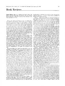
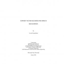
4. Simulation Results To illustrate the behaviour of the model and the stateestimation algorithms, the simulation results presented here have been carried out on a small corpus of acoustic data, and the articulatory interpretation of the hidden states is ignored at present, setting the observation function h(:) to be the identity mapping. The aim was to examine the data- tting capability of the model, and to determine the importance of the dierent parameters during estimation; computational burden precludes a full evaluation at present. Training and test data, each consisting of 100 hand-labelled words from a single speaker in the speaker-dependent portion of the DARPA Resource Management database, were parameterized using 12 mel-frequency cepstral coecients, calculated every 10ms using a 15ms Hamming window. Word models were constructed from phone transcriptions, sharing a set of 47 single-state phone models; each phone was represented by a second-order linear system with piecewiselinear target trajectories, with and without continuity constraints across boundaries. The models were initialized by training the target trajectories alone, and then re-trained using 10 iterations of the EM algorithm; v and w were xed throughout. Word labels were supplied during training, but without phone boundaries. During testing, the hidden X and U trajectories were estimated and compared with the original data. Figure 1 shows a typical result for the word \Tuscaloosa's"; Figure 2 shows the same data with continuity imposed on the U trajectory, but not its slope. The eect of allowing a distribution of targets is clear from the two dierent trajectories modelling the =s= phone. Imposing continuity constraints tends to make the U process model the data directly; when U is free to vary across boundaries it behaves like a true target, the X process models the dynamics, and the in uence of the system matrices is more pronounced. Figure 3 illustrates the eect of varying v for the word \Arkansas's", and demonstrates the importance of controlling this parameter carefully. As v is increased, the model interprets more of the signal variation as modelling error, and does not attempt to t it using the target process U . When v and w are trained, the eect of these parameters can often swamp the behaviour of the phonetic model. By adjusting the noise covariances, the model can be made to ignore a certain amount of global \non-linguistic" variation, sharpening the target distributions. A key feature of the model is that it provides a number of mechanisms for tting dierent sources of variation, each of which can be controlled and examined during training and recognition.

−−−−− U

C1 Value

0 −0.5 −1 −1.5 −2 −2.5 −3 0

20

40

60

80

100

Frame Index

Figure 1:

\Tuscaloosa's" : without continuity constraint. ....... Data;

− − − X;

−−−−− U

1 0.5 0

C1 Value

1. Ramsay G. and Deng L. Maximum-likelihood estimation for articulatory speech recognition using a stochastic target model. In Proc. Eurospeech-95, pages 1401{1404, 1995. 2. Russell M.J. and Moore R. Explicit modelling of state occupancy in hidden markov models for automatic speech recognition. In Proc. ICASSP-85, pages 2376{ 2379, 1988. 3. Deng L., Aksmanovic M., Sun D., and Wu J. Speech recognition using hidden Markov models with polynomial regression functions as non-stationary states. IEEE Trans. on Speech and Audio Proc., 2(4):507{520, 1994. 4. A fy M., Gong Y., and Haton J.-P. Stochastic trajectory models for speech recognition : an extension to modelling time correlation. In Proc. Eurospeech-95, pages 515{518, 1995. 5. Russell M. A segmental HMM for speech pattern matching. In Proc. ICASSP-93, pages 499{502, 1993. 6. Holmes W.J. and Russell M.J. Speech recognition using a linear dynamic segmental HMM. In Proc. Eurospeech95, pages 1611{1614, 1995. 7. V. Digalakis, J.R. Rohlicek, and M. Ostendorf. ML estimation of a stochastic linear dynamical system with the EM algorithm and its application to speech recognition. IEEE Transactions on speech and audio processing, 1(4):431{442, 1993. 8. Ross K. A dynamical system model for recognizing intonation patterns. In Proc. Eurospeech-95, pages 993{996, 1995. 9. Shumway R.H. and Stoer D.S. Dynamic linear models with switching. Journal of the American Statistical Association, 86(415):763{769, 1991. 10. Gordon K. and Smith A.F.M. Modelling and monitoring discontinuous changes in time series. In Spall J., editor, Bayesian Analysis of Time Series and Dynamic Models, pages 359{391. Marcel Dekker: New York, 1988. 11. Shirai K. and Honda M. Estimation of articulatory motion. In Dynamic Aspects of Speech Production. University of Tokyo Press, 1976.

− − − X;

0.5

−0.5 −1 −1.5 −2 −2.5 −3 0

20

40

60

80

100

Frame Index

Figure 2: SV=0.0001

6. REFERENCES

....... Data; 1

SV=0.01

The stochastic target model presented in [1] has been extended to include piecewise-deterministic control trajectories with continuity constraints. The optimal non-linear ltering and smoothing recursions required to estimate the hidden states of the model from acoustic data have been derived, and a sub-optimal approximation technique has been outlined. Preliminary data- tting experiments indicate that the model is capable of accounting for coarticulation across and within phone boundaries, and makes use of a number of different mechanisms for modelling possible sources of variability. Future work will compare the performance of the model on articulatory and acoustic recognition tasks.

12. Fujisaki H. Functional models of articulatory and phonatory dynamics. In Articulatory Modelling and Phonetics, pages 49{64. G.A.L.F., 1977. 13. Aggoun L., Elliott R.J., and Moore J.B. A measure change derivation of continuous state Baum-Welch estimators. Journal of Mathematical Systems, Estimation, and Control, 5(3):1{12, 1995. 14. Bar-Shalom Y. and Fortmann T.E. Tracking and Data Association. Academic Press, 1988.

SV=1.0

5. Conclusions

\Tuscaloosa's" : with continuity constraint. ....... Data;

− − − X;

−−−−− U

0 −2 −4

10

20

30

40

50

60

10

20

30

40

50

60

10

20

30

40

50

60

0 −2 −4 0 −2 −4

Frame Index

Figure 3:

Eect of v on state estimation.