Optimal Model Order Selection for Transient Error Autoregressive ...

World Academy of Science, Engineering and Technology 42 2008

Optimal Model Order Selection for Transient Error Autoregressive Moving Average (TERA) MRI Reconstruction Method Abiodun M. Aibinu, Athaur Rahman Najeeb, Momoh J. E. Salami, and Amir A. Shafie

Abstract—An alternative approach to the use of Discrete Fourier Transform (DFT) for Magnetic Resonance Imaging (MRI) reconstruction is the use of parametric modeling technique. This method is suitable for problems in which the image can be modeled by explicit known source functions with a few adjustable parameters. Despite the success reported in the use of modeling technique as an alternative MRI reconstruction technique, two important problems constitutes challenges to the applicability of this method, these are estimation of Model order and model coefficient determination. In this paper, five of the suggested method of evaluating the model order have been evaluated, these are: The Final Prediction Error (FPE), Akaike Information Criterion (AIC), Residual Variance (RV), Minimum Description Length (MDL) and Hannan and Quinn (HNQ) criterion. These criteria were evaluated on MRI data sets based on the method of Transient Error Reconstruction Algorithm (TERA). The result for each criterion is compared to result obtained by the use of a fixed order technique and three measures of similarity were evaluated. Result obtained shows that the use of MDL gives the highest measure of similarity to that use by a fixed order technique. Keywords—Autoregressive Moving Average (ARMA), Magnetic Resonance Imaging (MRI), Parametric modeling, Transient Error.

I. I NTRODUCTION

implementing the inversion formula, one focuses on finding an image function that satisfy the data consistency constrain [1]. Methods involve in MR reconstruction can broadly be divided into two namely: Non parametric and Parametric methods of MR reconstruction [4]. The use of Non-parametric technique such as the use of a two-dimensional discrete Fourier transform (DFT) as an MRI reconstruction technique has found common usage in the field of MRI. Despite the popularity of this technique,it still suffers from Gibb’s effect, introduction of artifacts and decrease in Spatial resolution. Parametric modeling technique is suitable for problems in which the image can be modeled by explicit known source functions with a few adjustable parameters [7]. In the field of MRI reconstruction, this involves modelling the rows or columns data of the acquired data points or in some cases model both the rows and the columns [1], [2], [4], [6], [8]–[10] as an image reconstruction scheme. The general principles governing the use of modeling techniques for image reconstruction are:

Magnetic Resonance Imaging (MRI) is used primarily in medical fields to produce images of the internal section of the human body [1]–[3]. The raw data or k-space data obtained, often made up of M x N e.g (256 x 128 ) complex valued data points. These data are reconstructed in order to obtain the final image called MR images. The basic MR reconstruction can be regarded as finding an image function P that is consistent with the measured signal S according to a known imaging equation S = f [P ]

P =f

S

•

•

•

(2)

In real life f [S] cannot be computed because of the nature of the data space which is partially sampled, instead of directly Athaur Rahman Najeeb is with the Kulliyah of Engineering, International Islamic University Malaysia (IIUM), email: [email protected] Momoh.J.E Salami is with the Kulliyah of Engineering, International Islamic University Malaysia (IIUM), email: [email protected] Amir A. Shafie is with the Kulliyah of Engineering, International Islamic University Malaysia (IIUM), email: [email protected] Abiodun. M. Aibinu, Malaysia, email: [email protected]

Sufficiency: The model must accurately represent the image. Efficiency (Parsimony): The model can characterized the image function with little parameters. Robustness: Must be stable in the face of perturbation and noise Computability: Efficient computations of parameters.

Signal modeling involves two steps, namely; 1) Model selection: Choosing an appropriate parametric form for the model data 2) Model Parameter determination: Model parameter determination include the determination of model order and model coefficients.

(1)

where f represent spatial information encoding scheme [1]. Furthermore, If f is invertible, a data consistent P can be obtained from the inverse transform such that −1

•

Successful application of modeling technique hinges on efficient method of model order determination. In this parametric MRI reconstruction, five known modeling technique have been evaluated. These are FPE, AIC, RV, MDL and HNQ. This paper is organized as follows; Section. I gives a brief introduction to MRI reconstruction and its associated terminology. Detail of steps involve in TERA reconstruction is as contained in section II. In Section. III various methods of model order determination would be discussed. Section. V and Section. V-B discusses the result obtained and conclusion respectively.

161

World Academy of Science, Engineering and Technology 42 2008

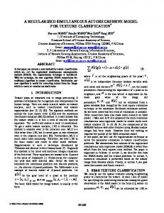
II. R ELATED W ORK The Transient Error Reconstruction Algorithm (TERA) involves modeling the data as a deterministic ARMA model with definite number of steps [4], [6]. The block diagram for this method is as shown in Fig. 1 and the steps involved is as discussed in subsection II-A

F T (xn ) =

•

F T (ǫn ) F T (an )

(8)

where 0 ≤ n ≤ ∞ where FT denotes Fourier Transform. Step - 4 The fourier transform of the original transform can now be calculated using S(ejω ) = 2{Re[F T (xn )] + jIm[F T (yn )]} − [s0 ] (9) where F T (xn ) and F T (yn ) are the fourier transform of the data sequences xn and yn respectively for, n ≥ 0. III. M ODEL O RDER D ETERMINATION M ETHODS

The model order determination methods evaluated in these paper are : FPE, AIC, RV, MDL and HNQ. • Final Prediction Error (FPE): FPE is a method of selecting the order of an AR model by minimizing the variance of the prediction error [15]. The function is given by N + (K + 1) (10) F P E(K) = σ 2 N − (K + 1) Fig. 1.

TERA Modeling Technique

where K is the model order, N is the number of data points and σ 2 is the total squared error divided by the number of data points, N. It is mathematically express as

A. Review: TERA Method Steps involve in TERA based MRI reconstruction are: • Step - 1: Split each row or column of the MRI data Sn into Hermitian or Anti-Hermitian series to account for data symmetry using Eq. 3 and Eq. 4

•

xn = (sn + s∗−n )/2

(3)

yn = (sn − s∗−n )/2

(4)

σ2 =

p X

ak x(n − k) + ǫ(n)

where L is the maximum of the order. ǫ is defined as ǫ(n) = x(n) − x ¯(n) where x ¯(n) is the predicted value of x(n) for order k By evaluating K from 1to L the optimal model , K is the one that gives the minimum value of FPE. That is F P E(p) = min(F P E[k]) (1 ≤ K ≤ m) •

the approximate equation function is given as

(5)

AIC(K) = N lnσ 2 + 2K

k=1

1+

1 p P

(6) •

ak z −k

k=1 •

Asymptotic Information Criterion (AIC): The Asymptotic Information Criterion (AIC) normally refer to as Akaike Information criterion is a measure of goodness of fit of an estimated statistic model [10], [16]. AIC reflects the balance between complexity of the model order and goodness of fit. This AIC method of order determination is given by, AIC(K) = N ln(maximumlikelihood) + 2K

with the transfer function given in (6) Y (z) H(z) = = X(z)

(K = 1, 2, 3, . . . , L)

K

where 0 ≤ n ≤ L − 1 Step - 2: Each series is modeled as the output of an IIR filter by estimating the transfer function from the finite data set. In order to achieve this, Smith et al determines the coefficients of the ARMA model by re-formulating the ARMA as a cascade of MA and AR filter. The single impulse δ(n) produces the data series ǫ(n) as the output of the filter HM A(z). The component series x(n) is modeled as the output of a pth order AR pole excited by ǫ(n). Thus, the component series can be model by the difference equation x(n) = −

N −1 1 X 2 ǫ N

The term 2K represents the penalty for selecting higher order. Minimum Description Length (MDL) The MDL is given by M DL(K) = N lnσ 2 + Kln(N )

Step - 3 The fourier transform is estimated from the AR and MA coefficient of the Hermitian and anti-Hermitian series. B(ejω ) (7) F T (xn ) = A(ejω )

(11)

(12)

This increases the penalty factor incur by using higher order as compared to AIC, thus favouring the selction of lower model order.

162

World Academy of Science, Engineering and Technology 42 2008

•

1) Mean Square Error (MSE) This involve computing the square of the difference between pixels in two different images and then taken the average over all pixels in the image. An image that is a perfect reproduction of the original image will have an MSE of zero, while an image that differs greatly from the original image will have a large MSE [19]. The equation for MSE is

Residual Variance (RV) The Residual variance criterion for order determination function is given by N −K σ2 (13) N − 2K − 1 This method work on the assumption that if the terms of AR or ARMA fitted is insufficient, the estimate of the variance will be increased by those terms not yet included in such a model [10]. HNQ This technique also counteract the over fitting nature of AIC. 2ln(lnN ) HN Q(K) = ln(σ 2 (K))) + K (14) N RV (K) =

•

M SE =

In TERA based MRI reconstruction [4], [6], The total forward error given by Ef =

n=p

|x(n) +

p X

ai xn−i |2

(16)

where M, N are the dimension of the image, P(x,y) is a pixel of the original image and Q(x,y) is the corresponding pixel from the reconstructed image. 2) Structural Similarity Index (SSI) The mathematically defined universal quality index [20] models any distortion as a combination of three different factors, namely a) Loss of correlation, b) Luminance distortion; c) Contrast distortion. The dynamic range of SSI is

IV. TERA O RDER D ETERMINATION AND I MAGE S IMILARITY MEASUREMENT

L−1 X

N M 1 XX |P(x,y) − Q(x,y) |2 M N y=1 x=1

(15)

SSI = [−1, +1]

i=1

The best value 1 is achieved if and only if the two images are similar and -1 if the two images are highly un-similar. 3) Correlation Co-efficient (CC) Correlation coefficient quantifies the closeness between two images. This coefficient value ranges from -1 to +1, where the value +1 indicates that the two images are highly correlated and are very close to each other. And the value -1 indicates that the images are exactly opposite to each other. The correlation coefficient is given by PM PN ¯ ¯

is minimized. In [4], the best way to determine the optimal order is to monitor Ef as the model order increases. When Ef shows a sharp decline, smith et al proposes that, such a point represent the correct model order. In a related work reported in [18], a simple plot of F P E(K) against model order K ( Fig. 2), shows that at the optimal model order, F P E(K) will be the minimum point and Ef will display a sharp decline. This method therefore make use of Eq. 10 in selecting the optimal model order.

x=1 qP M PN x=1

y=1

y=1

(P(x,y) − P(x,y) )(Q(x,y) − Q(x,y) )

(P(x,y) − P¯(x,y) )2

PM PN x=1

y=1

¯ (x,y) )2 (Q(x,y) − Q (17)

V. O BSERVATION AND C ONCLUSION A. Obeservation Table I and Table II shows result obtained using five of the model order determination technique to determine the optimal model order for the Hermitian and AntiHermitian components of the K-space data on a modeled row data respectively. The result shows similarity in the model order obtained by the use of FPE and AIC for all the rows. There are significant differences in the model order obtained by the use of any of the remaining three methods. The sixth column contain the data obtained by the use of fixed order value. Fig. 2.

Model Order using FPE and Ef (Plot source [18])

The result obtained for image similarity measure is as contained in Table III while the final images obtained is as shown in Fig. 3. Images obtained by the use of MDL method shows a great similarity to the fixed order type. The value obtained (0.9304) using SSI similarity measure technique is the highest among the evaluated methods, followed by the use of HNQ. FPE and AIC value are also similar though little improvement in FPE

A. Output Image Similarity measures In order to compare the result obtained, three objective image quality measured were used, these are Mean Square error, and Structural Similarity (SSI) and Correlation Coefficient (CC).

163

World Academy of Science, Engineering and Technology 42 2008

TABLE III M EASURE OF S IMILARITY USING DIFFERENT MODEL DETERMINATION

TABLE I M ODEL O RDER FOR H ARMITIAN M ATRIX Row Number 10 21 28 71 86 115 143 153 223 235 263 342 385 392 406 456 431 473 500 511 512

FPE

AIC

RV

MDL

HNQ

2 6 2 5 5 13 4 11 2 2 21 2 15 2 3 6 3 16 2 2 2

2 6 2 5 5 13 4 11 2 2 22 2 15 2 3 6 3 16 2 2 2

2 9 9 5 5 13 4 11 13 11 21 2 15 8 3 6 3 16 2 2 2

2 2 2 2 2 12 4 4 2 2 6 2 7 2 3 6 2 16 2 2 2

2 2 2 5 2 12 4 11 2 2 6 2 7 7 3 6 3 16 2 2 2

TABLE II M ODEL O RDER FOR A NTI H ARMITIAN M ATRIX Row Number 44 53 55 66 109 123 153 159 186 216 223 238 264 302 319 355 381 415 437 495

FPE

AIC

RV

MDL

HNQ

18 15 16 38 4 3 11 10 7 3 3 5 7 5 5 5 2 7 7 2

18 15 16 38 4 3 11 10 7 3 3 5 7 5 5 5 2 7 7 2

18 15 16 4 5 3 11 10 7 3 11 5 7 5 5 5 4 8 7 2

14 8 8 4 4 3 4 2 7 2 2 5 7 2 4 5 2 2 7 2

14 15 10 4 4 3 11 5 7 3 3 5 7 2 5 5 2 7 7 2

(0.9282) against AIC (0.9279) was obtained for this particular image. Furthermore, comparing the images obtained by the use of MSE, shows that MDL gives the least measure of error (67.6348) as compared to the value obtained by the use of FPE (90.6970) and AIC (90.6990). Lastly, MDL CC value 0f (0.9998) is the highest value compared to any of the other method with CC value of (0.9997). B. Conclusion In this paper, methods of determining optimal model order for MRI images reconstruction have been presented. The model orders were applied on real K-space data based on TERA MR reconstruction algorithm. Five criteria to determine the model order were evaluated in this work. The result shows that the value obtain for FPE and AIC for dynamic order

METHODS

Order Type FPE AIC RV MDL HNQ

SSI 0.9282 0.9279 0.9273 0.9304 0.9291

MSE 90.6970 90.6990 86.5087 67.6348 74.0820

CC 0.9997 0.9997 0.9997 0.9998 0.9997

determination are same for all rows of images, while the value obtained for other model order determining techniques were quite different. Furthermore, this work also shows that based on the use of measure of image similarity the value obtained for MDL shows similarity with that of using fixed order technique and will be more appropriate for model order determination for reconstruction of MRI data using TERA Algorithm. R EFERENCES [1] Z. P. Liang, P. C. Lauterbur, “Principles of Magnetic Resonance Imaging, A signal processing perspective”, IEEE Press, New York, 2000. [2] D. G. Nishimura, “Principles of Magnetic Resonance Imaging”, April 1996. [3] “MRI Basics: MRI Basics”. Accessed September 21, 2007, from Website: http://www.cis.rit.edu/htbooks/mri/inside.htm [4] M. R. Smith, S. T. Nichols, R. M. Henkelman and M. L. Wood, “Application of Autoregressive Moving Average Parametric Modeling in Magnetic Resonance Image Reconstruction”, IEEE Transactions on Medical Imaging, Vol. M1-5:3, pp 257 - 261, 1986. [5] F. J. Harris,“On the Use of Windows for Harmonic Analysis with the Discrete Fourier Transform”, Proceedings of the IEEE. Vol. 66, January 1978. [6] M. R. Smith, S. T. Nichols, R. Constable and R. Henkelman, “A quantitative comparison of the TERA modeling and DFT magnetic resonance image reconstruction techniques”, Magn. Reson. Med., Vol. 19 pp. 1-19, 1991. [7] R. C. Puetter, T. R. Gosnell, and A. Yahil “Digital image reconstruction: Deblurring and Denoising”, Annu. Rev. Astron. Astrophys., pp 43:139, 2005. [8] Z. P. Liang, F. E. Boada, R. T. Constable, E. M. Haacke, P. C. Lauterbur, and M. R. Smith, “Constrained Reconstruction Methods in MR Imaging”, Reviews of MRM, vol. 4, pp.67 - 185, 1992. [9] E. Hackle and Z. Liang, “Superresolution Reconstruction Through Object Modeling and Estimation”, IEEE transactions in A.S.S.P, 37: 592 - 595, 1989. [10] R. Palaniappan, “Towards Optimal Model Oreder Selection for Autoregressive Spectral Analysis of Mental Tasks Using Genetic Algorithm”, IJCSNS International Journal of Computer Science and Network Security, Vol. 6 No. 1A, January 2006. [11] Z. Wang, A. C. Bovik, and L. Lu, “Why is image quality assessment so difficult”, Proc. IEEE Int. Conf. Acoustics, Speech, and Signal Processing, vol.4, Orlando, FL, pp. 3313-3316, May, 2002. [12] T. Mathews Jr. and M. R. Smith, “Objective Image Quality Measures for Evaluating Advanced MRI Reconstruction Method”, Proc. of IEEE CCECE, pp. 396 - 361, 1996. [13] Z. Wang, A. Bovik, “A Universal quality index”, IEEE Signal Processing Letters, vol. 9, no. 3, pp. 8 1-84, March 2002. [14] Z. Wang, A. C. Bovik, H. R. Sheikh, and E. P. Simoncelli, “Image quality assessment:From error measurement to structural similarity”, IEEE Transactions on Image Processing, accepted for publication April 2003. [15] H. Akaike, “Power Spectrum Estimation through Autoregression Model Fitting”, Annals of the Institute of Statistical Mathematics, vol. 21, pp. 407-419, 1969. [16] H. Akaike, “A New Look at the Statistical Model Identification”, IEEE Trans. Autom. Control, vol. AC-19, pp. 716-723, 1974. [17] J. Rissanen, ”Modelling by shortest data description”, Automatica, vol.14, pp.465-471, 1978.

164

World Academy of Science, Engineering and Technology 42 2008

ARMA Image by FPE Model Order

ARMA Image by AIC Model Order

(a)

(b)

ARMA Image by RV Model Order

ARMA Image by MDL Model Order

(c)

(d) ARMA Image by HNQ Model Order

(e) Fig. 3. Image Reconstructed by the use of (a) FPE Model Order (b) AIC Model Order (c) RV Model Order (d) MDL Model Order (a) HNQ Model Order

[18] M.J.E Salami, A. R. Najeeb, O. Khalifa, K. Arrifin, “MR Reconsturction with Autoregressive Moving Average”, International Conference on Biotechnology Engineering, Kuala Lumpur, pp 676 - 704, May, 2007. [19] G. P. Mulopulos, A. A. Hernandez and L. S. Gasztonyi “Peak Signal to Noise Ratio Performance Comparison of JPEG and JPEG 2000 for Various Medical Image Modalities” , Symposium on Computer June, 2003. [20] B. Shrestha, C.G. O’Hara and N. H. Younan, “JPEG2000: IMAGE QUALITY METRICS”, ASPRS 2005 Annual Conference, Baltimore, Maryland March 7-11, 2005.

165