OPTIMAL TRANSIENT RESPONSE SHAPING IN MODEL

OPTIMAL TRANSIENT RESPONSE SHAPING IN MODEL PREDICTIVE CONTROL D.E. Davison ∗,1 R. Milman ∗∗ E.J. Davison ∗∗,1 ∗ University

of Waterloo, Waterloo, Ontario, Canada, N2L 3G1 of Toronto, Toronto, Ontario, Canada, M5S 1A4

∗∗ University

Abstract: This paper considers the problem of designing a multivariable model predictive controller (MPC) which results in a time response that is smooth, that has a desired speed of response, and that has small cross-channel interaction. This objective is satisfied, subject to fundamental limitations on achievable performance, by introducing a new cheap-control quadratic performance index that has the desired transient response characteristic embedded within it. Examples are included to show that minimizing the proposed performance index improves the transient response when compared to the c 2005 IFAC standard quadratic performance often used in MPC. Copyright Keywords: Predictive control, Cheap control, Transient responses, Multivariable control systems, Discrete-time systems, Linear control systems.

1. INTRODUCTION There is a huge literature on model predictive control (MPC), e.g., see (Garcia et al., 1989; Soeterboek, 1992; Rawlings, 1999; Camacho and Bordons, 1999; Mayne et al., 2000; Rawlings, 2000; Goodwin et al., 2001; Maciejowski, 2002; Keerthi and Gilbert, 1988; Milman and Davison, 2003b; Milman and Davison, 2003a) for some representative texts, survey articles, and recent papers on the topic. This paper considers the MPC tracking and regulation problem for a multivariable discrete-time linear shiftinvariant plant. Both the tracking reference signal (i.e., the desired set point) and the disturbance are assumed to be constant, although the disturbance is taken to be unknown and unmeasurable. The focus of the paper is on the transient performance aspects of controller design. Specifically, the goal is to design a MPC controller which solves the Robust Servomechanism Problem (reviewed in Section 2) and which, for the nominal plant, results in a “good” transient response in the sense that the closed-loop system response is

“smooth”, the speed of response is at a desirable level, and there are only “small” interactions between the outputs. Due to fundamental limitations of achievable performance described, for example, by Ben Jemaa and Davison (2003), one would expect that it is possible to meet these objectives in the case where the plant is minimum-phase. The performance index often used in MPC is a quadratic performance index, such as N

J=

∑

k=1




(1)

where e(k) := yref (k) − y(k) denotes the tracking error, Q > 0 is a scaling matrix (often chosen to be the identity matrix), and Φ(k) is some quadratic expression of the system’s control input signals. It will be shown in this paper that a significant improvement in transient response performance can be obtained if the performance index (1) is replaced by an alternate “cheap control” performance index of the form N

J=

∑ (z(k)0Qz(k) + Φ(k))

k=1

1

Funded by the Natural Sciences and Engineering Research Council of Canada (NSERC).

e(k − 1)0 Qe(k − 1) + Φ(k)

where

 θ θ e(k − 1) + e(k) z(k) := I − h h 

(2)

with the plant (3): 

and θ is a designer-specified diagonal matrix whose diagonal elements satisfy θi > h, where h is the designer-specified sampling period. This performance index was first introduced in (Davison and Davison, 2003), although not in an MPC context. 2. PRELIMINARY RESULTS Assume that the multivariable plant to be controlled arises from sampling a continuous-time plant with sampling period h > 0, and has the structure x(k + 1) = Ax(k) + Bu(k) + Ew(k) y(k) = Cx(k) + Du(k) + Fw(k)

(3)

e(k) = y(k) − yref (k)

      B x(k) A 0 x(k + 1) u(k) (5) + = D η(k) C I η(k + 1)    w E 0 + yref F −I      D C 0  x(k) +  0  u(k) ym (k) =  0 I  η(k) 0 0 0    F 0  w + 0 0  yref 0 I

where ym (k) are the measurable outputs of the system. It is shown in (Davison, 1996; Goldenberg and Davison, 1974) that if the conditions of Theorem 2.1 hold, then there exists a compensator which stabilizes (5); moreover, any compensator which stabilizes the augmented system (5) also solves the RSP.

where x(k) ∈ Rn , u(k) ∈ Rm , y(k) ∈ Rr , w(k) ∈ RΩ denote the state, control input, (measurable) output to be controlled, and (unmeasurable but constant) disturbance acting on the system, respectively. In addition, yref (k) ∈ Rr denotes the (constant) tracking reference signal, and e(k) ∈ Rr the tracking error in the system. The disturbance matrices E and F are not necessarily assumed to be known in the following development, so the results in this paper apply for arbitrary unknown (but constant) disturbances.

In the next section, we consider the problem of designing a compensator that, in addition to stabilizing the augmented plant and thereby solving the RSP, satisfies the objective of having a smooth time response whose speed can be set to any desirable value, and which has little cross-channel interaction.

At this point, it is instructive to review the Robust Servomechanism Problem (RSP), as described in (Davison, 1996). The RSP for (3) involves finding a linear shift-invariant controller which has inputs y(k), yref and output u(k) so that:

The goal of obtaining a “good” transient response will be achieved if the controller can force every element of the tracking error, e(k) = yref − y(k), to decay to zero at a pre-specified rate. With this in mind, introduce the diagonal matrix

(a) the resulting closed-loop system is asymptotically stable, (b) asymptotic tracking regulation occurs for the disturbance and tracking reference signals, i.e.

θ := diag(θ1 , θ2 , ..., θr ),

lim e(k) = 0, ∀x(0) ∈ Rn , ∀w ∈ RΩ , ∀yref ∈ Rr

k→∞

and for all controller initial conditions, (c) condition (b) holds for all perturbations of the plant model (e.g., plant parameters or plant dynamics including changes in model order) which do not cause the resulting perturbed closed-loop system to become unstable. The following existence result is well known (Davison, 1996; Goldenberg and Davison, 1974)): Theorem 2.1: There exists a solution to the robust servomechanism problem for plant (3) if and only if the following conditions are all satisfied: (a) (C, A, and detectable  B) is stabilizable A−I B = n + r. 2 (b) rank C D

(6)

where θi > h, i = 1, 2, ..., r determines the desired time constant for the ith channel, and introduce the following output:   1 1 z(k) := I − θ e(k − 1) + θe(k). (7) h h In terms of the variables z(k), x(k) ˆ := x(k) − x(k − 1), u(k) ˆ := u(k) − u(k − 1), and (from (4)) e(k) = η(k + 1) − η(k), a representation for the augmented plant (5) is 

      B x(k) ˆ A 0 x(k ˆ + 1) u(k) ˆ (8) + = D e(k − 1) C I e(k)    1 1 x(k) ˆ z(k) = θC I + θDu(k). ˆ e(k − 1) h h

The advantage of working with system (8) is that the unknown (but constant) external inputs do not appear. The following theorem relates properties of (8) to those of the plant (3) with w = 0, yref = 0:

Consider now the following augmented system formed by cascading the servo-compensator for (3), given by η(k + 1) = η(k) + e(k),

3. MAIN RESULTS

(4)

x(k + 1) = Ax(k) + Bu(k) y(k) = Cx(k) + Du(k).

(9)

Theorem 3.1: (a) The augmented plant representation (8) is stabilizable and detectable and possesses the same fixed modes as (9) if and only if the existence conditions of Theorem 2.1 both hold. (Fixed modes are those modes which are not both controllable and observable; see (Davison, 1996).) (b) The augmented plant representation (8) is minimum phase if and only if the plant (9) is minimum phase. 2 It follows from this theorem that if the plant (3) satisfies the RSP existence conditions, then there exists a controller (with input z(k) and output u(k)) ˆ that stabilizes (8). Moreover, any such stabilizing controller for (8) also solves the RSP for (3). 3.1 Proposed Performance Index and Controller Given the augmented system (8), consider the problem of finding a state-feedback controller u(k) ˆ = K0 x(k) ˆ + K1 e(k − 1)

controller (12) with parameters in (13)–(14) is applied to (8), the following closed-loop system response is obtained: e(k) = [I − hθ−1 ]k e(0), k = 0, 1, 2, 3, . . .

(15)

In other words, the error response has a smooth, exponentially-decaying behaviour. Moreover, since θ is a diagonal matrix, the closed-loop response is completely decoupled, where the ith diagonal element of θ determines the time constant of the ith channel. Of course, in practice it is not possible to use ε = 0, but if the plant is minimum-phase then, by continuity, ε can be chosen to be sufficiently small to guarantee performance arbitrarily close to that in (15). If the plant is non-minimum phase, the usual limitations on performance apply (e.g., see (Ben Jemaa and Davison, 2003)), so the ideal performance (15) is not achievable even as ε → 0; however, the motivation for (11) still remains, and, as shown later in an example, it is possible to improve the transient performance even in the non-minimum phase case.

(10)

which results in a stable closed-loop system and which brings about “good” transient error regulation. To achieve these objectives, it is proposed that the performance index ∞   ˆ , (11) Jproposed (k) := ∑ z0 (i)Qz(i) + εuˆ0 (i)Ru(i) i=k

be minimized, where ε > 0 is the “cheap control” parameter, Q > 0 and R > 0 are weighting matrices, and z is given by (7). Assuming that the existence conditions of Theorem 2.1 hold, it follows from Theorem 3.1 and standard LQR theory that there exists an optimal stabilizing controller which minimizes (11) subject to (8), and which solves the RSP for (3). In terms of u, the optimal state-feedback controller (10) can be written as

u(k) = u(k − 1) + K0 [x(k) − x(k − 1)] + K1 e(k − 1). (12) The motivation for choosing the performance index (11) is explained as follows. Suppose the plant (3) is minimum phase with m = r, D = 0, and that θi > h (i = 1, 2, . . . , r) in (6). Consider minimizing (11) as ε → 0, i.e., consider the use of cheap control. From (Ben Jemaa and Davison, 2003), it is determined that the controller which minimizes (11) as ε → 0 has the form of (10) (or, equivalently, (12)) with  −1   1 1 K0 = − θCB θCA +C , (13) h h  −1 1 K1 = − θCB , (14) h where the indicated inverses exist for almost all parameters of the continuous-time plant which gave rise to the plant (3); in particular, the inverses exist for all continuous plants which have a non-singular interactor matrix, which is the generic case. If the optimal

3.2 Addition of Control Signal Constraints and MPC Define the set o n ≤ ui ≤ umax , i = 1, 2, ..., m , U := u ∈ Rm umin i i (16) max , for i = 1, 2, ..., m. Let U ◦ denote where umin < u i i the interior of U. Consider now the plant (3) with the control constraint u(k) ∈ U. Assuming that the existence conditions of Theorem 2.1 hold, the results from (Miller and Davison, 1993) can be used to determine the feasibility of a given pair (yref , w) when constraint set (16) is invoked. In particular, define †    0 A−I B (17) T := [0 Im ] Ir C D  †   A−I B E U := − [0 Im ] , (18) C D F where (·)† = (·)0 [(·)(·)0 ]−1 . Then (yref , w) is feasible with respect to constraint set (16) if     yref T U ∈ U ◦. (19) w If (19) does not hold, then (at least, for the case m = r) there does not exist a control input that both lies in the constraint set (16) and achieves asymptotic tracking/regulation for the pair (yref , w). Assuming that the tracking reference signal and disturbance are feasible with respect to the constraint set (16) and that the conditions of Theorem 2.1 hold, the performance index Jproposed,MPC (k, N) =

k+N−1 

∑

i=k

z(i)0 Qz(i) + εuˆ0 (i)Ru(i) ˆ



(20)

results presented here, the MPC algorithm in (Milman and Davison, 2003b) was used for controller design.

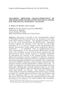
cart u

(a) flexible cable

mass y w

(b)

M K

K

The first example is a non-minimum-phase singleinput single-output flexible crane, pictured in Figure 1(a). The input is the force applied to the cart, and the output is the horizontal position of the mass. For certain masses, spring constants, etc., the basic equations of motion, linearized about the “down” equilibrium point and sampled with sampling period h = 0.1 seconds, fit a model of the form (3) where   1 0.1 0.04882 0.001628 0.0006816 0.0001857 0 1 0.9748 0.04882 0.08267 0.0004959     0 0 0.9902 0.09967 0 0 ,  A=  0 0 −0.1950 0.9902 0 0   0 0 0 0 0.7555 0.008402  0 0 0 0 −40.509 0.7471

Fig. 1. (a) Flexible crane system; (b) Multivariable mass-spring-damper system.

 5.0959 · 10−6 −4   1.0169 · 10    −4.9919 · 10−7    B= −6  ,  −9.9674 · 10   5.0705 · 10−7  8.4020 · 10−5   C = 1 0 0 0 0 0 , D = 0, E = 0, F = 0.

is proposed for implementation using MPC. In the MPC implementation, a quadratic programming algorithm is used to minimize the cost (20) subject to the control constraint u(k) ∈ U at every sample instant, and the control signal pertaining to the first sample is then implemented to control the plant. The performance index (20) is motivated by (11), where the only difference is that the horizon, N, is now finite. If N is sufficiently large and if the control signal constraint is inactive, then the optimal cost in (20) will be arbitrarily close to the optimal cost in (11), and the resulting controller will solve the RSP. If the control constraint is active (and assuming the disturbance and reference signal are feasible) the controller that minimizes (20) will still solve the RSP, but the optimal cost will be larger than the unconstrained optimal cost.

Figure 2 presents simulation results obtained when MPC is applied to the crane system for a unit step reference signal. The solid curves show the resulting behaviour when the proposed performance index (20) is used with ε = 10−5 , θ = 3, N = 100, corresponding to an ideal error transient that has a decaying exponential with a time constant of θ = 3 seconds. For comparison, the dashed curves in Figure 2 show the closed-loop behaviour when the “standard” performance index (21) is used with ε = 10−5 , N = 100. In both cases, state feedback is used to implement the control. Observe that the MPC controller using the proposed performance index gives a much smoother time response than that obtained using the “standard” performance index; moreover, the improved transients are obtained without using extra control effort.

The proposed performance index (20) is similar to standard quadratic MPC performance indices, for example,

Similar improvements are evident in the situation where the control signal is constrained. For example, Figure 3 shows the closed-loop behaviour under the constraint |u| ≤ 300 and Figure 4 shows the behaviour under the tighter constraint |u| ≤ 100. It is seen again that the MPC controller using the proposed performance index results in a much smoother time response compared to the “standard” performance index (21).

y1

Jstandard (k, N) =

k+N 

∑

i=k

B

B

m1

m2

u1

u2

y2

 e(i − 1)0 Qe(i − 1) + εuˆ0 (i)Ru(i) ˆ .

(21) The key difference between (20) and (21) is that z is penalized in the former, and e in the latter. As argued previously, and as exemplified below, penalizing z results in improved transient performance. 4. EXAMPLES We now illustrate the effectiveness of the proposed performance index using two examples. For all the



The second example is based on a minimum-phase multivariable mass-spring-damper apparatus, shown in Figure 1(b), where the system inputs are forces and the outputs are positions; there is also a disturbance force, w. Assume that the masses are M = 10 and m1 = m2 = 1, the spring constant is K = 1, the damper coefficient is B = 1, and the sampling period is h = 0.1. The resulting model has parameters

Position, y(k)

1 0.5

Control, u(k) [unconstrained]

0 0

5

10

15

20

25

15

20

25

Time (s) 500 0 −500 0

5

10 Time (s)

Position, y(k)

Fig. 2. Step response for the flexible crane system. The solid curves are for the proposed controller and the dashed curves are for the standard controller.

1 0.5 0 0

5

10

15

20

25

15

20

25

Control, u(k) [|u(k)| ≤ 300]

Time (s) 500 0

−500 0

5

10 Time (s)

Position, y(k)

Fig. 3. The same conditions as in Figure 2, except now the control signal is constrained by |u(t)| ≤ 300.

1 0.5 0 0

5

10

15

20

25

15

20

25

Time (s) Control, u(k) [|u(k)| ≤ 100]

9.990 · 10−1  −1.984 · 10−2   4.975 · 10−3 A=  9.920 · 10−2   4.975 · 10−3 9.920 · 10−2 

500 0

−500 0

5

10 Time (s)

Fig. 4. The same conditions as in Figure 3, except now the control signal is constrained by |u(t)| ≤ 100.

9.987 · 10−2 9.970 · 10−1 6.636 · 10−4 1.489 · 10−2 6.636 · 10−4 1.489 · 10−2

4.975 · 10−4 9.920 · 10−3 9.950 · 10−1 −9.927 · 10−2 2.070 · 10−6 6.610 · 10−5

6.636 · 10−5 1.489 · 10−3 9.934 · 10−2 9.851 · 10−1 2.568 · 10−7 8.680 · 10−6

 4.975 · 10−4 6.636 · 10−5 9.920 · 10−3 1.489 · 10−3   2.070 · 10−6 2.568 · 10−7  , 6.610 · 10−5 8.680 · 10−6   9.950 · 10−1 9.934 · 10−2  −9.927 · 10−2 9.851 · 10−1     5.00 · 10−4 2.076 · 10−6 2.076 · 10−6 −3 −5 −5  9.99 · 10   6.636 · 10 6.636 · 10       2.08 · 10−6   4.979 · 10−3 5.943 · 10−9      B= −5  , −2 −7  , E =   6.64 · 10   9.934 · 10 2.568 · 10   2.08 · 10−6   5.943 · 10−9 4.979 · 10−3  −7 −2 2.568 · 10 9.934 · 10 6.64 · 10−5   00 10 00 C= , D = 0, F = 0. 00 00 10 Figure 5 presents closed-loop simulation results obtained when MPC is applied with the reference signal yref = (1 0)0 and no disturbance. The solid curves correspond to the proposed performance index (20), with ε = 100, θ = 4, N = 100. The dashed curves correspond to the “standard” performance index (21) with ε = 100, N = 100. Again in both cases, state feedback is used to implement the control. Evidently the MPC controller obtained using the proposed performance gives a much smoother response with smaller crosschannel interaction compared to the standard performance index. Next, consider the same situation, but with control constraints |u1 | ≤ 0.5 and |u2 | ≤ 0.5. The simulation results are given in Figure 6. Note that the MPC controller using the proposed performance index again gives a smoother response with a significant reduction of cross channel interaction compared to the standard performance index (21). Finally, consider the closed-loop disturbance response for the mass-spring-damper system, shown in Figure 7. The parameters are the same as before, except yref is zero and the disturbance, w(k), is set to 1 at t = 5 and reset to 0 at t = 60; these times are indicated in the figure with arrows. There is also a mild control constraint: −0.75 ≤ ui ≤ 0.25, i = 1, 2. Note that, due to symmetry, y1 (k) = y2 (k) and u1 (k) = u2 (k). Although the behaviour of the proposed controller is similar to the standard controller, observe that the transient peaks are reduced. 5. CONCLUSIONS This paper has proposed a new type of cheap-control quadratic performance index for model predictive control. Taking into account limitations arising in the

0.2

y1(k)

0.5 y2(k)

0 0

5

10

15

20 Time (s)

25

30

35

u1(k)

0

u2(k)

−0.5 10

15

20 Time (s)

25

30

35

40

Position

1

y1(k)

0.5 y2(k)

0

Control [constrained]

5

10

15

20 Time (s)

25

30

35

40

35

40

1 0.5

u (k) 1

0 u (k) 2

−0.5 −1 0

5

10

15

20 Time (s)

40

60

80

100

60

80

100

0.5 0 −0.5 −1 0

20

40 Time (s)

Fig. 5. Step response for the mass-spring-damper system with yref = (1 0)0 . The solid curves are for the proposed controller and the dashed curves are for the standard controller.

0

20

Time (s)

0.5

5

0

−0.2 0

40

1

−1 0

0.1

−0.1

Control [constrained]

Control [unconstrained]

Position

Position

1

25

30

Fig. 6. The same conditions as in Figure 5, except now the control signals are constrained, |u1 (k)| ≤ 0.5 and |u2 (k)| ≤ 0.5. non-minimum phase case, minimizing this new index with a small enough ε results in a nominal transient response that has a desired speed of response, is “smooth”, and is “almost free” of interaction between output channels. It is also interesting to note that, for the examples presented, a significant improvement in transient performance (relative to the “standard” controller) can be attained without using significantly more control effort. REFERENCES Ben Jemaa, L. and E.J. Davison (2003). Performance limitations in the robust servomechanism problem for sampled LTI systems. IEEE Transactions on Automatic Control 48(8), 1299–1311. Camacho, E. and C. Bordons (1999). Model Predictive Control. Springer. Davison, D.E. and E.J. Davison (2003). Optimal transient response shaping for the discrete-time servo problem. In: 2003 European Control Conference. Cambridge, UK. 6 conference pages. Davison, E.J. (1996). Robust servomechanism problem. pp. 731–747. CRC Press and IEEE Press.

Fig. 7. Disturbance response of the mass-springdamper system subject to a control signal constraint. Garcia, C., D. Prett and M. Morafi (1989). Model predictive control: Theory and practice–a survey. Automatica 25(3), 335–348. Goldenberg, A. and E.J. Davison (1974). The feedforward and robust control of a general servomechanism problem with time lag. In: 8th Annual Princeton Conference on Information Science Systems. pp. 80–84. Goodwin, G., S. Graebe and M. Salgado (2001). Control Systems Design. Chap. 23. Prentice Hall. Keerthi, S. and E. Gilbert (1988). Optimal infinite horizon feedback laws for a general class of constrained discrete time systems: Stability and moving-horizon approximations. Journal of Optimization Theory and Applications 57, 265–293. Maciejowski, J. (2002). Predictive Control with Constraints. Prentice Hall. Harlow, England. Mayne, D., J. Rawlings, C. Rao and P. Scokaert (2000). Constrained model predictive control: Stability and optimality, survey paper. Automatica 36, 789–814. Miller, D.E. and E.J. Davison (1993). An adaptive tracking problem with a control input constraint. Automatica 29(4), 877–887. Milman, R. and E.J. Davison (2003a). Evaluation of a new algorithm for model predictive control based on non-feasible search directions using pre-mature termination. In: Proceedings of the Conference on Decision and Control. IEEE. pp. 2217–2221. Milman, R. and E.J. Davison (2003b). Fast computation of the quadratic programming subproblem in MPC. In: American Control Conference. pp. 4723–4729. Rawlings, J. B. (1999). Tutorial: Model predictive control technology. In: American Control Conference. San Diego. pp. 662–676. Rawlings, J.B. (2000). Tutorial overview of model predictive control. IEEE Control Systems Magazine pp. 38–52. Soeterboek, R. (1992). Predictive control: A unified approach. Prentice Hall. New York, NY.