proved parallel algorithm can be used to derive fast parallel algorithms for several of the applications we have considered so far , including k-nearest-neighbors.
Optimal Parallel All-Nearest-Neighbors Using the Well-Separated Pair Decomposition (Preliminary Version) Paul B. Callahan* Computer Science Department Johns Hopkins University Baltimore, MD 21218
Teng [12] have developed an optimal randomized parallel algorithm using substantially different techniques. Their computational model assumes that prefix sum can be performed in 0(1) steps. The algorithm we present here is, to our knowledge, the first optimal deterministic parallel algorithm for solving all-neatestneighbors, and requires O(1ogn) time with O ( n ) processors on a standard CREW PRAM. We have developed several additional applications of the well-separated pair decomposition [5, 71 and we feel it is of general utility in multi-dimensional proximity problems. Hence, we believe our results will be useful in the development of optimal parallel algorithms for many other problems posed on point sets in Rd. The well-separated pair decomposition of P consists of a binary tree whose leaves are points in P, and a list of pairs of nodes satisfying certain properties we will define later. In section 3, we present an improved parallel algorithm for constructing the tree. This algorithm requires several non-trivial techniques and will constitute the largest portion of the paper.' In section 4, we present an improved parallel algorithm for finding the pairs. In section 5, we show how our improved parallel algorithm can be used to derive fast parallel algorithms for several of the applications we have considered so far , including k-nearest-neighbors.
Abstract W e present an optimal parallel algorithm t o construct the well-separated pair decomposition of a point set P in Zd. W e show how this leads t o a deterministic optimal O(1ogn) t i m e parallel algorithm for finding the k nearest neighbors of each point in P, where k is a constant. W e discuss several additional applications of the well-separated pair decomposition for which we can derive f a s t e r parallel algorithms.
1
Introduction
In [5] we introduced the well-separated pair decomposition of a set P of n points in ?J?d, and showed how to apply this decomposition to develop efficient parallel algorithms for two problems posed on multidimensional point sets. One of these applications led t o the fastest known deterministic parallel algorithm for finding the k nearest neighbors of each point in P using O ( n ) processors. The time required for this algorithm is Q(log2 n), which is within a logn factor of the optima1,time complexity. In this paper, we close the gap by developing an optimal O(log n) time parallel algorithm for computing the well-separated pair decomposition. We have already shown that the k-nearest-neighbors problem can be solved in O(1ogn) time given the decomposition, so this result leads directly t o an optimal allnearest-neighbors algorithm. The k-nearest-neighbors problem has received a great deal of attention [3, 8, 10, 12, 16, 181. The first optimal sequential algorithm was presented by More recently, Frieze, Miller, and Vaidya [18].
2
We follow the conventions of [5], which we recall below. Let P be a set of points in Rd, where d is a constant denoting the dimension. We define the bounding 'A recent result of Bern et al. [4] on constructing quadtrees also leads to an optimal algorithm for this problem, but requires a more powerful machine mcdel in which certain logical operations can be performed on integer words. Our algorithm requires only algebraic operations, as is standard in computational geometry
*Supportedby the National Science Foundation under Grant
CCR-9107293.
0272-542&93 $03.00 0 1993 IEEE
Definitions
332
rectangle of P , denoted by R ( P ) , t o be the smallest rectangle that encloses all points in P , where the word “rectangle” denotes the Cartesian product R = [ X I ,z;] x [zz, 2/21x . . . x [ z d , z&] in 8’. We denote the length of R in the ith dimension by li(R) = z i - zi. We denote the maximum and minimum lengths by lmax(R) and lmin(R). When all l;(R)are equal, we say t’hat R is a d - c u b e , and denote its length by l ( R ) = l m a x ( R )= lmin(R).We write l ; ( P ) ,lmin(P),and l m a x ( P )as shorthand for l ; ( R ( P ) ) , lmin(R(P)),and lmax(R(P)),respectively. We say that point, sets A and B are well-separated if R(A) and R ( B ) can each be contrained in d-spheres of radius r whose distance of closest, approach is at least s r , where s is the s e p a r a t i o n , assumed t o be fixed throughout. our discussion a t a value strictly greater than 0. While we can define this notion in a somewhat more natural way without using bounding rect,angles, t,his definition will make subsequent. computation easier. We will often assume that, P has a binary tree T associated with it,, where each leaf of T is labeled by a singlet,on set containing one of t.he points in P , and each internal node is labeled by the union of all sets labelling the leaves of it,s subtree. We will refer t o each node in T by the name of the set labelling it. Since leaves are labeled by singleton sets, we may also refer t.0 them by the names of points. We define the i n t e r a c t i o n p r o d u c t , denoted 8 , bet,ween any two point sets A and B as follows:
A@
be a structure consisting of a binary tree T associated with P , and a well-separated realization of P 8 P that. uses T .
The tree we normally associate with the point set P will be of a special kind, which we call a fair split tree. To formalize this notion, we introduce some additional definitions. We define a split of P t o be its partition int’o two non-empt,y point sets lying on either side of a hyperplane (called the s p l i t t i n g h y p e r p l a n e ) perpendicular t o one of the coordinate axes, and not, intersecting any points in P . We define a split tree of P to be a binary tree, constructed recursively as follows. If IPI = 1, its unique split tree consists of the node P . Otherwise a split tree is any tree with root P and two subtrees that are split trees of the subsets formed by a split of P. For any node A in the tree, we denote its parent (if it exists) by d-4). We define the o u t e r rectangle of A, denoted R(A), for each node A top down as follows: 0
For the root P , let R(P) be an open d-cube centered at the center of R ( P ) , with l ( R ( P ) ) = lmax(P).
For all other A , the splitting hyperplane used for the split of p(A) divides R ( p ( A ) )into two open rectangles. Let R(A) be the one that contains A.
= { { P , P ’ } l P E A,P’ E B , a n d p # P’)
Note that P @P is the set. of all dist.inct pairs of points in P . A set, { { A l , B l } , .. . , { A k , B k } } of pairs of nonempty subsets of A and B is said t,o be a r e a l i z a t i o n of A@Bif
We define a f a i r split of A t o be a split of A in which the splitting hyperplane is at a distance of at least l m a X ( A ) / 3from each of the two boundaries of R ( A ) parallel’to it. A split tree formed using only fair splits is called a f a i r split tree. Intuitively, a fair split tree can be considered a variation of a quadtree (and its multidimensional extensions) in which the splitting conditions are relaxed so that a rectangle need not be split exactly in half in each dimension. This relaxed tree retains most of the useful properties of a quadtree, but it can be constructed efficiently in the algebraic model that is standard in computational geometry. We have shown [5] that given a fair split tree T , we can always construct a realization of P @ P containing O ( n ) pairs. We have presented a O ( n log n ) algorithm for constructing such a tree, which we have proven optimal, and an O(log2 n ) time parallel algorithm. We
i. A ; n B i = 0 f o r a l l i = 1, . . . , k ii. (A; 8 Bi) n (Aj @ B j ) = 0 for all i, j such that 1 l i < j < IC. k
iii. A 8 B = U A i 8
Constructing the fair split tree
3
B,
i=l
The realization is said t o be well-separated if it satisfies the additional property iv. Ai and Bi are well-separat.ed for all i = 1, . . . , IC Let T be the binary tree associated with P . For A,E P , we say that a realizat,ion of A 8 B u s e s T if all Ai and Bi in the realization are nodes in T . We define a well-separated p a i r d e c o m p o s i t i o n of P t,o
333
now consider the problem of constructing such a tree optimally in O(1og n) time in parallel. We use the technique of multiway divide-andconquer [2], in which a problem of size n is split into a set of subproblems, each of size O ( n a )for some a < 1. This approach cannot be applied in an obvious fashion, since we must preserve the fair-split condition during the “divide” phase of our algorithm. For example, it will not suffice t o .iivide the point set using hyperplanes in one dimension, since this may violate the fair-split condition. Instead, we must develop a nontrivial splitting phase that constructs a partial fair split tree whose leaves are rectangles, each containing O ( n Q )points. This phase makes heavy use of the relaxed nature of the fair-split condition as contrasted with the less flexible characterization of quadtrees.
3.1
invariants with respect t o the rectangles we consider
1. In each dimension, at least one side of R lies on a slab boundary. 2. For all i = 1 , . . . , d , either li(R’) = li(R) or l;(R’) 5 $Ii(R)
3. imin(R) 2 $Imax(R). We now consider the three cases of our splitting rule. For the following, we use ,,i t o denote the longest dimension of R. The application of our splitting rule will be said t o produce one or two new rect,angles that must preserve the above invariants. In our illustrations, slab boundaries are shown with thin dotted lines, while each rectangle and its corresponding split are shown with thick solid lines. Although only planar rectangles are illustrated, the formal splitting rules extend t o all d 2 1. Case 1: Imax(R)= limsx(R’) (see figures 1 and 2). In this case, both sides of R in the ,,i dimension lie on slab boundaries. We find the slab boundary in this dimension that comes closest t o splitting R into two equal halves. If (a) it lies at a distance of at. least ilma(R) from the closest side of R in the ,,i dimension, we use it for our split. Otherwise (b), we dimension. split R into two equal halves in the ,,,i This case produces two rectangles, each lying on one side of the split. Note that if case 1 does not hold, then by the second invariant,
The constructible rectangles
We begin by splitting our point set into slabs in each 1 axis-parallel hyperplanes, dimension, using [nl-.l spaced so that each slab contains a t most ne points. We will refer t o these hyperplanes as slab boundaries. Recall that the definition of a fair split allows some freedom in the choice of the splitting hyperplane. In the present algorithm, we will use the slab boundaries t o guide our choice of splits, thus limiting the kinds of rectangles that appear as nodes in the tree. In particular, we will be able t o represent each side of a rectangle by a constant-size arithmetic expression in terms of slab boundaries and small integers. We will later show how t o choose a t o substantially limit the number of constructible rectangles. This will be essential in maintaining a reasonable processor bound. Given a rectangle for which certain properties hold, we will develop a way of splitting it that results in new rectangles that preserve these properties and are constructible in sense we will later make precise. In certain cases, we will not be able t o split the rectangle, and must instead “shrink” it t o a much smaller rectangle sharing a corner with the original and containing all but O ( n Q )of the points in the original. This will lead t o a special compressed edge in the resulting tree. After we have finished constructing the tree, we will expand each compressed edge into a chain of splits using a technique developed in our previous parallel algorithm [5]. Finally, we will remove any rectangles that do not contain points, thus completing the splitting phase. Let R be a rectangle that we wish t o split. For the remainder of this discussion, let R’ denote the largest rectangle that is contained in R and whose sides lie on slab boundaries. We will maintain the following
+
We will assume this inequality holds in the remaining cases. In the following, c is a constant whose value we will determine later. Case 2: lmax(R’)2 clmax(R) (see figures 3 and 4). Exactly one of the sides of R in the ,,i dimension lies on a slab boundary, which we denote by H . If (a) li,=(R’) 2 $lmax(R), we use the hyperplane containing the side of R’ farthest from H for our split. Otherwise (b), we must choose another split which preserves our invariants. It is sufficient t o use a hyperplane splitting R at a distance from H in the interval ( f ,$]l,,(R). We find the unique integer j such that ~2 (4 5j l max(R‘) ) lies in the interval, and use a hyperplane at this distance. For technical reasons, we say that this case produces only one rectangle, namely the one containing R’. The other rectangle may be important in the tree we will ultimately construct, but we must defer its treatment t o a later phase, because it will violate the first invariant after an application of case 2(b).
334
I
I I I I
I I I
I I I I
I I I I
I I I I
I I I I
I I I I
I
I
I
I
I
I
I
I I I
I
I I I
I I I
I 1 I
I I
I I
I
I
I
,
I I
I I I
Figure 1: Case l(a)
I
I
I
I
I I I
I I I
I I I I -I-----I I I I I I
_--
Figure 3: Case 2(a)
I I I I
I I I I
I I I I I
I
1
I I I I
I I I I
I I I I I I
1 1 I
I I I
I I I
I I I
I I I
II I I I 1 I I I
,
I
I
I
I ,
- - - - -r - r - -
_ - - - - - - - - -_ - - - - - -r - I I I
I I I
I I
--I
Figure 2: Case l ( b )
Figure 4: Case 2(b)
Case 3: lmax(R’) < clmax(R)(see figure 5). For sufficiently small values of c , exactly one side of R lies on a slab boundary in each dimension. In other words, R’ shares a unique corner with R. We construct a dcube C containing R’ such that l ( C ) = $lmax(R’) and C shares the same corner with R as R’. We will later show how t o find a sequence of fair splits decomposing the region between R and C into rectangles that ) This case produces the rectancontain O ( n @ points. gle C . We must prove that the above cases preserve the invariants. The first invariant follows immediately from the fact that we never split R’ unless both sides parallel t o the split lie on slab boundaries. The third invariant follows from the fair split condition. That is, after the split, the new minimum length cannot be less than ilmax(R), while the new maximum length
cannot be more than Imax(R).The second invariant is somewhat more complicated t o verify. If we split on a slab boundary, the invariant is clearly preserved. Otherwise, all slab boundaries passing through R in dimension must be at a distance of less than the,,i ilmax(R)from the sides parallel t o them. Given this fact, it is not hard t o see that our choice of a splitting hyperplane in cases 1 and 2 preserves the invariant. It is even easier t o verify the invariant in case 3. In the above cases, the new rectangles produced by a split can always be encoded in terms of a constantsize list of slab boundaries and O( 1) bits of extra information. We will consider case 2(b) in some detail, because it is the most complex and allows the greatest number of new rectangles t o be defined. Suppose some dimension of a rectangle has been generated by an invocation of case 2(b). To fully spec-
335
I I I I I
I I I I I
Let T, be a subtree of G consisting of the nodes accessible from some initial rectangle Ro. We make the exception that a rectangle intersected by exactly two slab boundaries in the,,i dimension will be considered a leaf. Ro will normally be inherited from a previous phase in the algorithm, so the third invariant will be guaranteed automatically (initially, we use some dcube that contains the entire point set). To guarantee the first and second invariants, we set the extreme slab boundaries so that they contain the sides of the start,ing rectangle. For convenience, we may refer to nodes and rectangles interchangeably. It is hard to see how to construct T, without finding a transitive closure of G. We cannot rely on a general transitive closure algorithm, since this would be too time consuming. Fortunately, the structure of G is very restricted due t o the following property: Let U and v be two distinct nodes in G. If there exists a directed path from U to w , then this path is unique. In fact, given U and some v accessible from U , we can find the first arc along the path in constant time using the following observation:
I I I I I
I I I
II
I
I ,
II II
Figure 5: Case 3
ify this dimension, we must supply a slab boundary for one side of the rectangle, and a distance of the form 2 4 31 a( 3) max(R'), from which we may compute the position of the other side. We may represent this distance by the two slab boundaries that determine lmax(R'), and an integer j . We consider the possible values for j . Recall that the distance we represent must lie in the interval $lmax(R).We know that cl,,(R) 5 &,,,(RI) < lmax(R),and the right-hand side immediately gives us j 2 0. From the left-hand side, one may easily verify that j 5 -llogc/log QJ. Since c is a constant, there are 0(1)choices of j . It is easy t o see that rectangle dimensions generated by other cases of the splitting rule can be treated in a similar manner. For example, the hyperplane splitting a rectangle into two equal pieces in case l ( b ) can be represented as the arithmetic mean of two slab boundaries. An upper bound on the number of rectangles, valid to within a constant factor, may be obtained by considering only those rectangles whose dimensions come from case 2(b), since other cases result in fewer new rectangles. There are O ( T Z ' - ~slab ) boundaries, and at most 3d slab boundaries are required to represent a rectangle. This gives us the following result.
Observation 1 If there i s a directed path from U t o v i n G,then the first arc in the path i s the unique arc (U,w), such that ( U , w) i s an arc in G and the rectangle w contains the rectangle U.
(4,
Consider the graph GI, which contains a node [U, w] for each pair of nodes in the production graph G. Let. there be an arc from [U, U] t o [w,U] iff (U,w ) is an arc in G and v is contained in w. Nodes in G' have outdegree of at most 1 by the observation that ( U , w ) is unique. Hence, GI is a forest of rooted trees in which each node that is not a root has an arc leading to its parent. Each node of the form [U,U ] is the root of some tree, and clearly v is accessible from U in G iff [U,w] is a node in this tree.
3.3
Recall that for each U , we are ultimately interested in determining whether it is accessible from Ro in G. In other words, we wish t o know whether the tree rooted at [U,U ] contains the node [Ro,U]. With this observation, we are ready t o present the complete algorithm for computing T,:
Lemma 1 There are O ( T Z ~ ~ ( ' -constructible ")) rectangles. 0
3.2
Extracting T,
The production graph
1. Construct slabs in each dimension.
Consider the directed graph in which each node corresponds t o a constructible rectangle, and arcs are placed from each node t o any node it- can produce by an invocation of the splitting rule. We call such a graph a production graph and denote it by G.
2. Construct G from slab boundaries.
3. Construct G' from G. 4. Use G' to find v in G accessible from Ro.
336
Finally, T, consists of those v accessible from Ro, together with their out-going arcs. Correctness of the above algorithm follows from the preceding discussion. We now consider the parallel complexity of each step. Step 1 can be solved in the time it takes to sort the points in each dimension. This can be done with n processors in O(1ogn) time on an EREW PRAM [9]. Step 2 can be solved by assigning a processor to each possible formula for constructing a rectangle, so there are O( IGl) processors. Each processor can find an explicit value for its rectangle in constant time, and compute its out-going arcs in O(1ogn) time using a binary search on a sorted list of slab boundaries in the appropriate dimension. Step 3 can be solved in constant time once we have assigned a processor to every ordered pair of nodes in G. Each processor finds the out-going arc, if it exists, of the corresponding node in G’. Step 4 can be solved in several ways. Our approach is as follows. Assign a weight of 1 to all nodes in G’ of the form [Ro,v] and a weight of 0 to all other nodes. Now compute, for every node in G’, the total weight of its subtree. The computed total for [v,v] will be 1 iff [ R o , ~is] a node in its subtree, or equivalently, v is accessible from Ro in G. This can be solved in O(1og IGl) time with O( [GI2/log !GI) processors on an EREW PRAM using the Euler tour technique [17]. According to Lemma 1 , IGI = O(n3d(’-”)). Hence, then IGI2 = O ( n ) . if we choose some a 2 1 Therefore, the above algorithm requires O(1og n ) time with O ( n ) processors.
to continue our algorithm into the next phase. The fact that there are only O(fi) constructible rectangles allows us to solve this problem in O(1ogn) time on an EREW PRAM using a relatively simple algorithm. The details will be given in the final version. We must further process T, by expanding each edge produced by case 3 into a chain of splits. In presenting this part of our algorithm, we will derive the value of the constant c used in distinguishing cases 2 and 3. Let R be a rectangle in T, with child C produced by case 3. Construct the unique cube C’ such that l(C’) = $lmin(R),and C’ shares a corner with both C and R. Find a sequence of splits from R to C’ using a rule similar to case 1 in the preceding algorithm. Note that C’ is sufficiently small to guarantee that such a sequence is possible, and sufficiently large to guarantee that only 0 ( 1 ) splits are necessary. Hence, this can be done in constant time with one processor per rectangle R. Now we need only find a sequence of fair splits between C’ and C . Let m be the number of points inside C‘ and outside C . We have shown [5] how to find such a sequence of fair splits in O(1ogm) time with O(m) processors. As a precondition, we require that l(C’) 2 ! l ( C ) . We must choose c consistent with this constraint. Recalling that l ( C ) = Zimm(R’),we obtain the equivalent constraint lmin(R)2 %lmax(R’). By the third invariant in our splitting rule, lmin(R)2 ilmax(R).Hence, if we let c = then the precondition on case 3 guarantees that the constraint is satisfied. If we expand all the compressed edges concurrently, then the total number of processors assigned cannot exceed O ( n ) ,and the time will be O(1ogn). To complete the splitting phase, we compress out, any rectangles in the tree that do not contain points in the initial point set. This can be done as follows: Weight each leaf with the number of points contained in its rectangle. For each internal node, compute the total weight of the leaves in its subtree, and weight it with this value. Eliminate all nodes with weight zero, and compress non-branching paths to single edges. Before compression, the tree cannot have size greater than O(n). To see this, note that there were only O(fi) nodes before the expansion of case 3 edges, and any new rectangles generated by this expansion were guaranteed to contain points. Hence, compression can be performed in O(1ogn) time with O ( n ) processors on an EREW PRAM using standard techniques.
&,
&,
3.4
Constructing the partial fair split tree
We define a p a r t i a l f a i r split tree to be a tree that satisfies all the conditions of a fair split tree, except that its leaves need not be singleton point sets. In this section, we show how to construct a partial fair split tree from T,. First, recall that case 2 actually resulted in two rectangles, though we said it produced only one. This was necessary because the other violated the first invariant. To correct this problem, we treat the other as a leaf. We insert all such leaves in constant time by assigning a processor to every rectangle R with a child produced by case 2. At this point, the tree we have constructed defines a natural partition of the initial point set into points contained either in leaf rectangles, or else lying in the region between R and C in the nodes produced by case 3. We will need to compute this partition explicitly
331
3.5
Correctness of the splitting phase
1 (the precise value may be chosen to optimize the constants in the complexity). For n less than some constant no, solve the problem by brute force. Otherwise, construct a partial fair split tree Tp, whose leaves are point sets of size O(na). Find fair split trees for these point sets by applying the algorithm recursively in parallel. The point sets at the leaves form a partition of P, so the total number of processors remains O ( n ) at all stages of the recursion. The total time T ( n ) satisfies the recurrence T(n)5 p l o g n y T ( n Q ) for suitable choices of p and y. From this, it is easily seen that T ( n )= O(1ogn).
We use Tp to denote the tree ultimately constructed by the previous algorithm, and we wish t o show that Tp is a partial fair split tree. Note that after the final compression, every leaf of Tp contains a non-empty point set, and every non-leaf node containing the point set P has two children formed by a split of P. It suffices to prove that such splits are fair. We may focus our attention on those splits produced by cases 1 and 2 of the first part of the algorithm. Every node that is split in such a manner is labeled by a rectangle R, and it may be easily verified that the split is placed at a distance of a t least ilmax(R)from the nearest boundary of R parallel to the split. Because R contains P, lmax(R) _> lmm(P). Moreover, the outer rectangle R(P) contains R, so the nearest boundary of R(P) is no closer to the split than the nearest boundary of R. Thus it follows that each such split is fair, and Tp is a partial fair split tree. To prove the correctness of the splitting phase, we must finally argue that each leaf of Tp contains O ( n a ) points. We should emphasize that the number of leaves in Tp will not necessarily be O ( ~ Z ' - ~ ) .In fact, we may create linearly many new leaves when we break up case 3 edges into chains of fair splits. It suffices to show that the outer rectangle of every leaf lies entirely within two adjacent slabs in some dimension, since each slab contains nQ points. This can be verified by considering all the termination conditions that result in leaves. Note that the precise sequence of splits used in expanding case 3 edges is not important, because any rectangle in the region inside R and outside C must lie in two adjacent slabs. Other cases are even easier to verify. From the above discussion, we have the following lemma:
+
4
Given the point set P , let T denote a fair split tree of P. We consider the problem of computing the wellseparated pairs of the nodes of T . The pairs we compute will be the same as those produced by our sequential algorithm [5]. In the previous paper, we showed how to compute these pairs in O(log2n) time with O(n) processors, and in this section, we improve the time bound to O(log n) using the same number of processors. Roughly speaking, the sequential algorithm works by taking a pair (A, B) of nodes in T that are not wellseparated, forming two pairs by splitting the node with the larger bounding rectangle into its two children, and applying the process recursively until the result is a set of well-separated pairs. The initial pairs are all pairs of siblings in T . The pairs produced by this algorithm can be characterized as the set of all {A, 8)such that A and B are nodes in T with the following properties: A and B are well-separated, p(A) and B are not well-separated, and lmm(B) < imax(p(A))5 lmax(p(B)). For the leftmost inequality, we assume that some consistent method of tie-breaking is used in cases of equal lengths. The correctness of this characterization will be proven in the final version. The idea behind our parallel algorithm is to retrieve the set of pairs {A, B} simultaneously for all A. To do this, we develop a way to enumerate all B for any given A in O(1og n) time with one processor. Consider the problem of retrieving, for an arbitrary query cube C , all of those npdes B in T such that lmin(R(B))5 61(C) 5 lmin(R(p(B)))for some constant 6, and the outer rectangle R(B) overlaps C. Using a packing argument similar t o that given in [5], we can show that the number of such B is bounded by a function of 6 and d, and is thus a constant. To enumerate all B paired with a given A, we construct a suitably large cube C around p(A). We then
Lemma 2 Let P be a set of n points in ?I?', and let a be a real number in the interval [l- &, 1). In O(1ogn) time with O(n) processors on an E R E W P R A M , we can construct a partial fair split tree Tp of P such that each leaf of Tp contains O ( n Q )points. 0
3.6
Computing the pairs
The final algorithm
The above result leads directly to the following theorem.
Theorem 1 Let P be a set of n points in ?I?'. W e can find a fair split tree of P in O(1ogn) time with O ( n ) processors on an E R E W P R A M . Proof. Our algorithm is as follows: Let a be some constant greater than or equal to 1 and less than
&
338
solve the preceding problem for some 6, dependent upon s, and obtain a set of size O(1) that contains all B paired with A . From this set, the pairs { A , B } can be found in constant time by brute force. We now show how to solve the preceding problem in O(1ogn) time using one processor. We use a tree contraction technique such as rake and compress [15] or the centroid decomposition [ll] to construct a balanced tree partition T' such that the subtree of any node in T' is a tree partition of the nodes in some subtree of T from which at most one node and its subtree have been removed. Because T' is balanced, its depth is O(1ogn). Note that the union of all outer rectangles of nodes in a subtree of T' consists of a rectangle containing at most one rectangular hole (i.e., the outer rectangle of t.he missing subtree). We assume that each node in T' is labeled with such a geometric region. Given a node in T ' , we can therefore determine in constant time whether the outer rectangle of one of its descendants overlaps C . To retrieve the set of B that overlap C and satisfy the size condition, we begin at the root of T' and only descend into subtrees corresponding to a sufficiently large region that overlaps C . Every node at which we terminate this search process then corresponds to some B. We can determine all B in this manner, since we only skip nodes that are guaranteed not to contain such a B in their subtree. The subtree we traverse has a constant number of leaves and a depth no greater than the depth of T',which is O(1ogn). Hence, the t.ime to perform the search is O(1ogn). We can find T' in O(1og n) time with O ( n / log n) processors on an EREW PRAM [ll, 151. After constructing T', we assign a processor to each node A in T , and perform the preceding search process for each A simultaneously. This may result in concurrent reads, so we must use the stronger CREW model. Therefore, the complete algorit.hm requires O(1og n) time with O ( n ) processors on a CREW PRAM. Combining this with the result of the previous section, we obtain the following t.heorem. Theorem 2 Let P be a set of n points in 8 '. We can find a well-separated pair decomposition of P in O(1ogn) time with O ( n ) processors on a CREW PRAM. 0
5
Applications
Our primary application is the k-nearest-neighbors problem. We have already shown [5] that given a well-separated pair decomposition of a point set P ,
we can retrieve the k nearest Euclidean neighbors of each point in P for any constant k in O(1ogn) time with O ( n ) processors on an EREW PRAM. To do this, we parallelize our sequential algorithm using rake and compress [I, 13, 151. In this algorithm, we compute for each point x, a set of O( 1) candidates that may have x as one of its k nearest neighbors. This requires O(1og n) time with O ( n / log n) processors. We then extract the set of k nearest neighbors of each point, in O(1ogn) time with O ( n ) processors. By set,ting k equal to one, assuming all interpoint distances are distinct, we obtain an optimal parallel algorithm for the all-nearest-neighbors problem. The algorithm can be trivially modified to eliminate the assumption of distinct distances. Often, we may be interested in the dependence on k in the complexity. In the revised version of our previous paper [6], we presented a sequential algorithm that solved the k-nearest-neighbors problem in O(n1ogn kn) time. This is opt,imal with respect. to dependence on k. The corresponding parallel algorithm requires O(1og n) time with O ( k n ) processors on a CREW PRAM, and its work bound is therefore within a min{k, logn} factor of the optimal work bound. Other applications [5] include a parallel version of the Fast Multipole Method [14] for computing potential fields. Given the well-separated pair decomposition of a point set representing a charge distribution, we can implement the Fast Multipole Met.hod in O(1ogn) time with O(n/logn) processors on an EREW PRAM. Using our improved parallel algorithm for computing the decomposition, t,he total t.ime t.o solve this problem is now O(1ogn) witch O ( n ) processors. In [7], we presented several new applications of the well-separated pair decomposition. The algorit.hms we presented were sequential, but the basic techniques we employed can be parallelized using rake and compress on the decomposition tree. This leads to O(1og n) time algorithms for finding an €-approximate minimum spanning tree of P as well as an 6-appr0ximat.e complete Euclidean graph, or spanner. For const.ant. 6 , t.he work bounds are optimal.
+
References [l] K. Abrahamson, N. Dadoun, D. A. Kirkpatrick, and T. Przytcka. A simple parallel tree contraction algorithm. Journal of Algorithms, 10(2):287302, 1989.
M. J . Atallah and M. T. Goodrich. Efficient parallel solutions t o some geometric problems. Journal of Parallel and Distributed Computing, 3:492-507, 1986.
J. L. Bentley. Multidimensional divide-andconquer. CACM,23( 4):214-229,1980.
M. Bern, D. Eppstein, and S.-H. Teng. Parallel construction of quadtrees and quality triangulations. In Algorithms and Data Structures, Third Workshop, WADS '93, Lecture Notes an Computer Science 709, pages 188-199. SpringerVerlag, 1993. P. B. Callahan and S. R. Kosaraju. A decomposition of multi-dimensional point-sets with applications t o k-nearest-neighbors and n-body potential fields. In Proc. 24th Annual Symposium on the Theory of Computing, pages 546-556, 1992.
P. B. Callahan and S. R. Kosaraju, A decomposition of multi-dimensional point-sets with applications t o k-nearest-neighbors and n-body potential fields. Revised Version, 1992. P. B. Callahan and S. R. Kosaraju. Faster algorithms for some geometric graph problems in higher dimensions. In Proc. 4th Annual Symposium on Discrete Algorithms, pages 291-300, 1993. K. L. Clarkson. Fast algorithms for the all nearest neighbors problem. In Proc. 24th Annual Symposium on Foundations of Computer Science, pages 226-232, 1983.
[9] R. Cole. Parallel merge sort. SIAM Journal on Computing, 17:770-785, 1988. [lo] R. Cole and M. T. Goodrich. Optimal parallel algorithms for polygon and point-set problems. In Proc. 4th ACM Symp. on Computational Geometry, pages 201-210, 1988. [11] R. Cole and U. Vishkin. The accelerated centroid decomposition technique for optimal parallel tree evaluation in logarithmic time. Algon'thmica, 3:329-346, 1988. [12] A. M. Frieze, G. L. Miller, and S.-H. Teng. Separator based parallel divide and conquer in computational geometry. In Proc. 4th Annual symp. Parallel Algorithms and Architectures, pages 420429, 1992.
[13] H. Gazit, G. L. Miller, and S.-H. Teng. Optimal tree contraction in the EREW model. In S. K. Tewsburg, B. W. Dickinson, and S. C. Schwartz, editors, Concurrent Computations, pages 139155. Plenum Publishing, 1988. [14] L. F. Greengard. The Rapid Evaluation of Potential Fields an Particle Systems. The MIT Press, 1988. [15] S. R. Kosaraju and A. L. Delcher. Optimal parallel evaluation of tree-structured computations by raking. In J. Reif, editor, VLSI Algorithms and Architectures: Proceedings of the 3rd Aegean Workshop on Computing, pages 101-110. Springer-Verlag, 1988. [16] G. L. Miller, S.-H. Teng, and S. A. Vavasis. A unified geometric approach to graph separators. In Proc. 32nd Annual Symp. Found. Comp. Sc., pages 538-547, 1991. [17] R. E. Tarjan and U. Vishkin. Finding biconnected components and computing tree functions in logarithmic parallel time. SIAM Journal on Computing, 142362-874, 1985. [18] P. M. Vaidya. An optimal algorithm for the allnearest-neighbors problem. In Proc. 27th Annual Symp. Found. Comp. Sc., pages 117-122, 1986.