The Mitchell-Netravali filters [8] are also popular as ..... Figures 4(a) and (b) are as sharp as Figures 5(g)â¼(i), but their aliasing effect is slightly less severe.
Optimal Polynomial Filters Submitted to Journal of Graphics Tools
Zhouchen Lin
Hai-Tao Chen Heung-Yeung Shum Jian Wang Microsoft Research, Asia {zhoulin|i-htchen|hshum|jianw}@microsoft.com
Abstract In this paper, we present a family of circular or square optimal polynomial filters for pre-filtering 2D polygons and images. The criterion of designing polynomial filters is to maximize the energy concentration within a period of the spectra of the filters. The filters are non-negative and can have arbitrary radius and order. For a given radius, the filters converge very fast when the order increases, making low-order filters suffice for high-quality pre-filtering. With polynomial filters, it is convenient to evaluate the integral over the parts of polygons within the filter mask with closedform solutions, or generate look-up tables quickly via analytic evaluation. The experiments demonstrate the excellent anti-aliasing performance of our polynomial filters.
1 Introduction Anti-aliasing is a fundamental problem in computer graphics, in which choosing a good low-pass filter is critical to remove undesirable artifacts. Filter design has a long history in signal processing. For eliminating high frequencies, it is well known that the sinc function is the ideal filter. Unfortunately, it is of infinite support and is unusable in practice. Therefore, people have been searching for its alternatives. As simple filters can save much computation, box, conical, Gaussian, and cubic (including splines) filters are commonly used in computer graphics, either explicitly or implicitly. McCool proposed prism splines [7], but the evaluation is very complex and expensive. The Mitchell-Netravali filters [8] are also popular as people have found that they have good anti-aliasing performance [2, 4, 3]. The practitioners usually choose among the above-mentioned filters via visual examination on the rendered results. Therefore, the chosen optimal filter might be biased towards the experimental examples and be subjective. This paper is motivated by our work on a high-quality pre-filtering algorithm for 2D polygons [6], which evaluates the integral inside the filter mask by breaking the integral region into basic component regions bounded by a polygon edge, a radius passing one of the edge ends and the filter boundary. Our goals are to have filters that objectively minimize aliasing, and that can provide closed-form solutions to or generate a look-up table analytically for the basic component integral, i.e., the integral over the basic component region. We have developed a family of circular or square low-order polynomial filters that maximize the energy concentration in a period of their spectra. These filters can be used for pre-filtering polygons as presented in [6], and for processing discrete images as will be illustrated in this paper.
2 Filter Design We follow two criteria to design filters. First, the filter should minimize aliasing. Second, it must provide closed-form solutions to the basic component integral when a look-up table is not preferred. For the first criterion, we have to measure the “amount” of aliasing. It is well known that after sampling, the spectrum of a continuous signal replicates in the spectral domain. When the sampling is on a 2D square grid, the period is 2Ω = 2π/T in both x and y directions, where T is the sample spacing in the spatial domain, normalized to 1 in our problem. The amount of aliasing can be measured by the energy of the spectrum outside the square Ω = [−Ω, Ω] × [−Ω, Ω] in the spectral domain. Therefore, we should make the spectral energy most centered on the square. This leads to an
1
optimization problem:
� h = arg max � h
�
Ω
Ω
|[F (h)](ωx , ωy )|2 dωx dωy
−Ω ∞
�−Ω ∞
−∞
−∞
|[F (h)](ωx , ωy )|2 dωx dωy
,
(1)
where [F (h)] denotes the Fourier transform of the filter h. This is similar to the aliasing energy in [5]. The difference is that we use a ratio instead. Without any constraint, the solution to (1) is the well-known sinc function and the energy concentration is 1. However, in practice we want the filter be finitely supported. Under such a constraint, the solution to (1) becomes the prolate spheroidal wave function of order zero [9]. Unfortunately, the prolate spheroidal wave functions do not have closed-form solutions, even power-series solutions are unavailable. For the second criterion, among all elementary functions, only polynomials are possible to have closed-form solutions to the basic component integral. Following the above considerations, we design optimal polynomial filters, either square or circular, respectively. We only present these two types of filters because they are most commonly used. However, the same idea is applicable to other shapes of filters.
2.1 The optimal circular polynomial filters For circular polynomial filters, we may assume that h(r, θ) = numerator of (1) is given by � ΓΩ ≡
Ω −Ω
�
Ω
−Ω
M � k=0
hk rk , where r ∈ [0, R] and θ ∈ [0, 2π). Then the
|[F (h)](ωx , ωy )|2 dωx dωy =
M �
hk hl Ψkl ,
k,l=0
where
� Ψkl =
Ω
−Ω
�
Ω
−Ω
ψk ψl dωx dωy ,
and ψm is the Fourier transform of r m (0 ≤ r ≤ R): � ψm (ωx , ωy ) =
0
R
r
m+1
� dr
2π
0
e
−ir(ωx cos θ+ωy sin θ)
� dθ = 2π
R
0
rm+1 J0 (r|ω|)dr,
� in which J0 (·) is the 0-th order Bessel function and |ω| = ωx2 + ωy2 . By Parseval’s theorem on Fourier transform, the denominator of (1) is given by � Γ≡
∞
−∞
�
∞
−∞
� |[F (h)](ωx , ωy )|2 dωx dωy = (2π)2
∞
−∞
where
� Φkl =
0
2π� R 0
�
∞
−∞
rk+l+1 drdθ =
|h(x, y)|2 dxdy = (2π)2
M �
hk hl Φkl ,
k,l=0
2πRk+l+2 . k+l+2
The maximization of γ = Γ Ω /Γ can be achieved by utilizing the Lagrangian multiplier: ∂(ΓΩ − λ(Γ − 1)) ∂(ΓΩ − λ(Γ − 1)) = 0. = 0, and ∂hk ∂λ
(2)
This leads to an eigenvector problem: Φ−1 Ψh = λh, T
and h Φh = 1, 2
(3) (4)
Filter Type Radius h0 h1 h2 h3 Energy Concentration Maximum Energy Concentration
Table 1: Some data on low-order polynomial filters. Circular Square 1 2 1
2
0.56904256713865
0.26412404360302
0.71247167744650
0.45090000658189
0.05056692464147
−0.03455158299490
−0.79090785614255
−0.22055267318930
−0.91026906187835 0.42672641722501
−0.15934681709384 0.05631744983035
0.25582137300511
0.02911569510537
0.93801371604876
0.99950079154631
0.96260897769620
0.99888861744658
0.93801385499638
0.99965857174068
0.96261252017346
0.99988655625306
0.25
0.6
0.2
0.5
0.15
0.4
0.1
0.3
0.05
0.2
0.1 −1
−0.8
−0.6
−0.4
−0.2
0
0.2
0.4
0.6
0.8
0 −2
1
−1.5
−1
(a)
−0.5
0
0.5
1
1.5
2
(b)
Figure 1: The central cross sections of the circular polynomial filters. (a) Filters with radius 1, where the top, middle and bottom curves correspond to M = 1, M = 2 and M ≥ 3, respectively. (b) Filters with radius 2, where the bottom, top and middle curves correspond to M = 1, M = 2, and M ≥ 3, respectively. Note that the curves for M > 3 are nearly indistinguishable from that for M = 3. where Φ = (2π)2 (Φkl ), Ψ = (Ψkl ), and h = (h0 h1 · · · hM )T . For maximization, h must be chosen as the eigenvector that corresponds to the maximal eigenvalue of Φ −1 Ψ and be normalized according to (4). Though the energy concentration improves when M increases, the convergence to the maximum energy concentration is very fast, especially when R ≤ 2. Because polynomials can approximate arbitrary continuous functions uniformly, the fast convergence indicates that our low-order optimal polynomial filters are actually very close to the prolate spheroidal wave function. Our numerical computation shows that M = 3 is enough for the corresponding filter to achieve over 99.98% of the maximum energy concentration at a given radius, achieved by the prolate spheroidal wave function. Figure 1(a) is the central cross section of the optimal circular filters with R = 1, where the top, middle and bottom curves correspond to M = 1, M = 2 and M ≥ 3, respectively. We can see that the curves for M > 3 are nearly indistinguishable from that for M = 3. Similar results are observable in Figure 1(b), where R = 2. The coefficients of the optimal circular polynomial filters at different radius are listed in the left part of Table 1. Now we give the closed-form solution to the basic component integral. For circular filters, the basic component region is shown in Figure 2(a). By defining a new coordinate, where the t-axis is along the marching direction of the polygon edge so that the interior is on the right hand side of the edge and the d-direction is π/2 behind the t-direction, the basic component region can be parameterized by the coordinate of the polygon vertex V in the new coordinate, i.e., the distance d from the pixel center to the polygon edge and the distance t between the vertex V and the projection of the M � hk Ik (d, t), where Ik (d, t) is the integral of center onto the polygon edge. The basic component integral is I(d, t) = k=0
3
y
y ymax
R V
y0
d
d
t
t
V
min
O
R
O
x
x0
(a)
yminx
(b)
Figure 2: The basic component region (shaded area) is bounded by one polygon edge, one radius passing the polygon vertex and the filter boundary. (a) For circular filters, the parameterization (d, t) is 2D. (b) For square filters, the parameterization (θ, d, t) is 3D. rk over the same region. Converting to polar coordinates (Figure 2(a)), we have 1 : � Ik (d, t) =
�
φ
φmin
dξ
R d cos ξ
rk+1 dr
� φ � � 1 Rk+2 − dk+2 (cos ξ)−(k+2) dξ k + 2 φmin � 1 � k+2 = (φ − φmin ) − dk+2 [Pk+2 (φ) − Pk+2 (φmin )] , R k+2
=
�
where φ = arctan(t/d), φmin = − arccos(d/R), and Pk (ξ) =
(cos ξ)−k dξ.
By partial integral, Pk (ξ) can be computed via the following recursion: Pk (ξ) =
1 k−2 (tan ξ)(cos ξ)−(k−2) + Pk−2 (ξ). k−1 k−1
2.2 The optimal square polynomial filters For square polynomial filters, it is easy to see that h(x, y) must be symmetric with respect to lines x = 0, y = 0, and M M � � y = x. Therefore, we may assume that h(x, y) = hpq x2p y 2q , with hpq = hqp , where |x|, |y| ≤ R. Then p=0 q=0
� ΓΩ ≡
Ω
−Ω
�
Ω
−Ω
[F (h)](ωx , ωy )|2 dωx dωy =
M �
hpq hkl Ψ2p,2k Ψ2q,2l ,
p,q,k,l=0
where
� Ψ2m,2n =
Ω
−Ω
ψ2m ψ2n dω,
and ψ2m is the Fourier transform of x 2m (|x| ≤ R): � ψ2m (ω) =
R
−R
x2m e−ixω dx.
By partial integral, ψ 2m (ω) can be computed via the following recursion:
2(Rω)2m−1 2m cos(Rω) − ψ2m−2 (ω). ψ2m (ω) = R sin(Rω) + (2m)! ω 1 For
√ simplicity we do not discuss all possible (d, t), such as the case where d > R or t < − R2 − d2 . Section 2.2 also follows this convention.
4
The computation of Γ is similar, where Ψ 2m,2n changes to � Φ2m,2n =
∞
−∞
[F (x2m )](ω)[F (x2n )](ω)dω = 2π
�
R
−R
x2m x2n dx =
4πR2(m+n)+1 , 2(m + n) + 1
in which Parseval’s theorem is applied again. Utilizing the Lagrangian multiplier as in (2), we have: ΨHΨ = λΦHΦ, and trace(HΦHΦ) = 1,
(5) (6)
where Φ = (Φ2i,2j ), Ψ = (Ψ2i,2j ), H = (hij ), and trace(X) is the trace of matrix X. Equation (5) can be rewritten as: (A ⊗ A)vec(h) = λ · vec(h), ˜ where A = Φ−1 Ψ, ⊗ is the Kronecker product [1] of matrices, and vec(X) is the vectorization [1] of matrix X. Let λ ˜ M )T be the corresponding eigenvector, then λ ˜ 2 is the maximum ˜1 · · · h ˜ = (h ˜0 h be the largest eigenvalue of A and h ˜h ˜ T ) is the corresponding eigenvector ([1], more general theorem exists). Therefore, eigenvalue of A ⊗ A and vec( h ˜ is normalized via h ˜ T Φh ˜ = 1. This leads to a separable 2D filter ˜h ˜ T , where h we may choose separable H = h M � ˜ k x2k . h(x, y) = h(x)h(y), where h(x) = h k=0
Again, the convergence of h(x) is fast when M increases. Our numerical experiments show that M = 2 is sufficient for the corresponding filter h(x, y) to achieve over 99.9% of the maximum energy concentration when R ≤ 2. The coefficients of h(x) are listed in the right part of Table 1. For square filters, the basic component region is shown in Figure 2(b), where an extra parameter θ, which is related to the polar sweep angle of the d-axis, is required for the parameterization. The basic component integral is I(θ, d, t) = M M � � hmn I2m,2n (θ, d, t), where I2m,2n (θ, d, t) is the integral of x2m y 2n over the basic component region. Due to m=0 n=0
symmetry, we may assume that d ≥ 0 and 0 ≤ θ ≤ π/4. Breaking the basic component region into two shaded regions shown in Figure 2(b), we have �y0 I2m,2n (θ, d, t)
=
y dy ymin
=
�R
2n
2m+1
2m
x d−y sin θ cos θ
2n+1 (ymax
y�max
y 2n dy
dx + y0
2n+1 ymin )
�R
x2m dx
αy
2m+1
2(m+n+1) (ymax
2(m+n+1)
α − − y0 ) − (2m + 1)(2n + 1) 2(2m + 1)(m + n + 1) 2m+1 2n+k+1 2n+k+1 � − ymin 1 k k k 2m+1−k y0 , − (−1) C (sin θ) d 2m+1 (2m + 1)(cos θ)2m+1 2n + k + 1 R
k=0
where = d sin � θ + t cos θ, x0 d − R cos θ , −R , ymax ymin = max sin θ x0 n , Cm α = y0 y0
=d �cos θ − t sin θ, max {min{R/α, R}, −R} , if x0 > 0, = R, if x0 ≤ 0, m! . = n!(m − n)!
3 Experimental Results Figure 3 shows a wheel and a checkerboard rendered by our rendering system 2 , SplitRender [6], using the square polynomial filter with radius 2. There are 180 triangles in Figure 3(a), while Figure 3(b) has 92,100 quadrilaterals, 2 The
full-resolution images for Figures 3∼5 are available online at http://www.acm.org/jgt/papers/LinEtAl04.
5
(a)
(b)
Figure 3: The rendering results of SplitRender using the square polynomial filter with radius 2, closed-form solution used. most of which are extremely small and are at the top of the image. The rendering results are almost aliasing-free. For comparisons of our polynomial filters against various filters when pre-filtering polygons, please see [6]. Our polynomial filters can also be applied to filtering images. We now compare the anti-aliasing performance of various filters over discrete images. The test image is Figure 3(a) and will be scaled down by 1.8 times using various filters. The chosen filters include: square polynomial filters (M =2), circular polynomial filters (M =3), square Gaussian filters, circular Gaussian filters, conical filters, box filters and the Mitchell-Netravali filters [8]. The radii of the former 6 kinds of filters can be either 1 or 2, while those of the Mitchell-Netravali filters can only be 2. For Gaussian filters, we change σ from 0.1 to 1.2 to find the best filtering results, which should have good balance between eliminating aliasing and keeping the image sharp. For Mitchell-Netravali filters, the chosen (B, C) are: (1/3, 1/3), (0, 1), and (0, 0.5), respectively, as they have been mentioned in the literature [2, 4, 3]. The resultant images are computed via the following formula: � h(m ˜ − p, n ˜ − q)It (m, n) Ir (p, q) =
||(m−p,˜ ˜ n−q)||≤R
�
||(m−p,˜ ˜ n−q)||≤R
h(m ˜ − p, n ˜ − q)
,
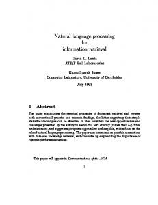
where It and Ir are the test image and resultant image, respectively, (m, ˜ n ˜ ) is the coordinate of pixel (m, n) of image It in image Ir , and � x2 + y 2 , if the filter is circular, ||(x, y)|| = max{|x|, |y|}, if the filter is square. Figures 4 are closeups of the down-scaling results of filters with radius 1, where σ = 0.3 for Gaussian filters. We see that square and circular polynomial filters (Figures 4(a) and (b)) result in least aliasing. The performance of square Gaussian (Figure 4(c)), circular Gaussian (Figure 4(d)) and conical filters (Figure 4(e)) is very close, and the box filter (Figure 4(f)) is the worst. Figures 5 are closeups of the down-scaling results of filters with radius 2, where σ = 0.9 for Gaussian filters. We see that square and circular polynomial filters and square Gaussian filters (Figures 5(a)∼(c)) have the least aliasing. Circular Gaussian (Figure 5(d)) and conical filters (Figure 5(e)) come next, and again the box filter (Figures 5(f)) is the worst. The results of Mitchell-Netravali filters (Figures 5(g)∼(i)) are very close to each other. They look sharper than the other images but their Moir´e patterns are also more severe. It is interesting to compare them with our polynomial filters with
6
(a)
(b)
(c)
(d)
(e)
(f)
Figure 4: Closeups of downscaling Figure 3(a) by 1.8 times using various filters with radius 1. (a) Square polynomial filter. (b) Circular polynomial filter. (c) Square Gaussian filter with σ = 0.3. (d) Circular Gaussian filter with σ = 0.3. (e) Conical filter. (f) Box filter. radius 1 (Figures 4(a) and (b)). Figures 4(a) and (b) are as sharp as Figures 5(g)∼(i), but their aliasing effect is slightly less severe. From the above comparisons, and from the polygon-filtering comparisons in [6], we may draw the following conclusions: 1. Our low-order optimal polynomial filters do have excellent anti-aliasing performance. 2. The anti-aliasing performance of our polynomial filters with radius 1 is comparable with that of the MitchellNetravali filters, which has a radius 2 and negative lobes. This makes our polynomial filters with radius 1 very useful because, without sacrificing performance, smaller radius often saves computation and at the same time its non-negativity can avoid the problems of clipping and ringing artifact that may result from the negative lobes of other filters. 3. Filters using closed-form evaluation are more suitable for high-quality anti-aliasing. Using look-up tables or super-sampling always introduces random noise if the sizes of graphical objects are beyond their precision. 3
References [1] Yun-Peng Cheng, Kai-Yuan Zhang, and Zhong Xu. Matrix Theory (in Chinese). Northwest Industrial Undersity Press, Xi’an, Shaanxi, China, 2000. 3 This
is a conclusion in [6].
7
[2] Tom Duff. Polygon scan conversion by exact convolution. Raster Imaging and Digital Typography ’89, pages 154–168, 1989. [3] A. E. Fabris and A. R. Forrest. Antialiasing of curves by discrete pre-filtering. In SIGGRAPH 1997 Conference Proceedings, Annual Conference Series, pages 317–323, August 1997. [4] Brain Guenter and Jack Tumblin. Quadrature prefiltering for high quality antialiasing. ACM Trans. on Graphics, 15(4):332–353, 1996. [5] J. Kajiya and M. Ullner. Filtering high quality text for display on raster scan devices. In SIGGRAPH 1981 Conference Proceedings, Annual Conference Series, pages 7–15, August 1981. [6] Zhouchen Lin, Hai-Tao Chen, Heung-Yeung Shum, and Jian Wang. Pre-filtering 2d polygons without clipping. Journal of Graphics Tools, ??(??):??, 2004. [7] M. D. McCool. Analytic antialiasing with prism splines. In SIGGRAPH 1995 Conference Proceedings, Annual Conference Series, pages 429–436, August 1995. [8] Don P. Mitchell and Arun N. Netravali. Reconstruction filters in computer graphics. In SIGGRAPH 1988 Conference Proceedings, Annual Conference Series, pages 221–227, August 1988. [9] D. Slepian and H. O. Pollak. Prolate spheroidal wave functions, fourier analysis and uncertainty —1. The Bell System Technical Journal, 40:43–64, 1961.
8
(a)
(b)
(c)
(d)
(e)
(f)
(g)
(h)
(i)
Figure 5: Closeups of downscaling Figure 3(a) by 1.8 times using various filters with radius 2. (a) Square polynomial filter. (b) Circular polynomial filter. (c) Square Gaussian filter with σ = 0.9. (d) Circular Gaussian filter with σ = 0.9. (e) Conical filter. (f) Box filter. (g) Mitchell-Netravali filter with B = 1/3, C = 1/3. (h) Mitchell-Netravali filter with B = 0, C = 0.5. (i) Mitchell-Netravali filter with B = 0, C = 1.
9