Discriminant Filters For Object Recognition. Owen Carmichael, Shyjan Mahamud, Martial Hebert. Technical Report CMU-RI-TR-02-09. The Robotics Institute.
Discriminant Filters For Object Recognition Owen Carmichael, Shyjan Mahamud, Martial Hebert Technical Report CMU-RI-TR-02-09 The Robotics Institute Carnegie Mellon University Pittsburgh, PA 15213
Abstract This paper presents a technique for using training data to design image filters for appearance-based object recognition. Rather than scanning the image with a single set of filters and using the results to test for the existence of objects, we use many sets of filters and take linear combinations of their outputs. The combining coefficients are optimized in a training phase to encourage discriminability between the filter responses for distinct parts of the object and clutter. Our experiments on three popular filter types show that by using this approach to combine sets of filters whose design parameters vary over a wide range, we can achieve detection performance competitive with that of any individual filter set. This in turn can ease the task of fine-tuning the settings for both the filters and the mechanisms that analyze their outputs.1
Figure 1:
Example images with object parts labelled.
one or more filters. A common paradigm is to first gather up example image patches containing the parts and run them through the filters; the filters can then be applied to a novel image and their responses compared to those for the training views to check for part matches. Filter sets appropriated for this purpose include convolutional kernels like Gabor wavelets [2] [13][18] and Gaussian derivatives[18][2][17], differential invariants based on combining the outputs of those kernels [19], local eigenspaces/PCA [5][10][15], and color statistics[22]. Each contains distinct characteristics that make them advantageous; for example, Gabor kernels are well-localized in space and frequency, invariants can tolerate transformations of the image, and local eigenspaces minimize reconstruction error of the training views.
1. Introduction In recent years, local-appearance-based approaches to object recognition have shown great potential to solve detection and pose estimation problems because they combine the modelling simplicity of global-appearance-based methods [14] with the robustness they lack. An object is represented by the appearances of its parts2 in a set of labelled training images (Figure 1); finding the object in a novel view begins with search for image patches containing the component parts (Figure 2). After these sections of object have been found, their relative positions in the image gives evidence to the pose of the object [21] or the likelihood that the part detections were spurious [3]. In many approaches, component appearance is represented by the responses of image windows containing it to
But none of these filters are designed from the beginning with component detection in mind. Those relying on pre-defined banks of kernels or statistics are not necessarily tuned to the appearances of specific objects and environments, so if the design parameters of the kernels are not properly set, it is possible that filter responses from distinct object parts will be indistinguishable from each other, or that outputs for background clutter will be the same as those for the object to be searched for. Local eigenspaces, although derived directly from training views, are not neccessarily tuned for discriminability either– they maximize the pooled covariance of all example patches of all object components, but do not necessarily encourage discriminability
1 This
work was supported by NSF Grant IIS-9907142. this paper, we use the terms “part,” “component,” and “section” to refer to any small piece of surface on the object, not its functional components (i.e. limbs, joints, etc.) For example, each of the labelled rectangles in Figure 2 frames the image of what we call an “object part.” The term “patch” always applies to images, not 3D surfaces. 2 Throughout
1
between the different components and background. As a result, implementations rely on two types of optimizations: tuning the design parameters of the filters so that outputs for distinct parts are distinct, and adjusting the settings of the classification mechanism that decides which filter outputs at run-time correspond to which sections of object. For example, suppose we want to recognize objects by using image responses to a set of Gaussian derivatives to tally votes for object parts in a hash table, as in [17]. For some recognition scenarios it may be unclear how to determine what Gaussian standard deviation (later referred to as the “width” or “scale” of the kernel) will result in responses that are wellclustered for the same component and well-separated for different components; it may also be difficult to determine how to size the bins in the hash table to minimize incorrect votes. There are two common solutions to this problem. First is to discretize the range of reasonable filter parameter settings, run recognition experiments using each setting in turn, and select the setting which gives the best performance. Second is to generate filter responses over many parameter values for the same image patch at training time and/or run time. As an example of the second approach, Schiele et al [18] gather responses of training patches to Gaussian derivatives or Gabor kernels at several scales offline and compare these to the outputs for a single scale on a new image. Local eigenspace techniques, on the other hand, tend to take the first approach, generating filter responses for a single parameter setting for training and testing[5][10][15]. We show experimentally that by optimizing linear combinations of filter sets over a range of filter parameters we can achieve good part detection performance without requiring a suite of trial-and-error experiments or training a classifier with multiple distinct sets of responses per patch. Furthermore, we demonstrate that in some cases, the resulting filters can enhance classification to a degree that enables simpler classification mechanisms at run-time. We emphasize that this paper does not propose a new functional form for image filters; rather, we introduce a way to use training data to automatically combine sets of filters of any type in a way that enhances detection. We call the resulting filters discriminant filters because the combining coefficients are optimized to discriminate between responses for distinct object parts and clutter. As an example, to design the Gaussian derivative kernels mentioned earlier we would synthesize many filter sets, one for each choice of Gaussian width over a range of plausible values. We then compute the responses of the training patches to each of the filter sets, and determine what the coefficients of a linear combination of those filter sets should be so that the responses for different object parts are discriminated from each other, while responses for the same part
Figure 2: Detection of a subset of the parts from Figure 1 and clutter (marked “C”) in a novel image. For display purposes, we only searched for six of the 11 labelled sections on this side of the mug. The number of rectangles around each component is proportional to the confidence in its classification. Note that the window on the upper left portion of the mug is not mislabelled as clutter; since none of the components of interest are on that portion of the object, it is technically “clutter” for parts detection purposes. Results for detection of the complete set of mug parts using the approach described in this paper are presented in Section 4. are tightly clustered. The discriminant filter in this case is the result of combining the Gaussian derivatives using those coefficients. A survey of related approaches to filter design is in Section 2, followed by the formulation of discriminant filters in Section 3. Detection experiments which apply discriminant filters to three previously reported image filters are described in Section 4 and discussed in Section 5.
2. Previous Work
���������� � � ������� ����� � ������� ��� � �$!
To describe the problem setting more formally, we start with sets of example image patches corresponding to views of different object sections. We denote a set of image filters as a function which maps a -dimensional space of image patches of fixed size to the -dimensional space of filter outputs. Our recognition paradigm is to compute for all and use these outputs to train a classifier to correctly detect when novel responses corresponding to image patches contain some object part. This section reviews previous designs for and the classifier. Several authors, including [5], [15], [20], and [10] propose the use of principal components analysis to model the local appearances of components, much the way earlier researchers [12] [14] modelled global appearances. An eigenspace decomposition is computed for the set of all training patches (or Fourier transforms of them as in [10]), and run-time parts detection consists of projecting novel image windows onto the first several significant eigenvectors. Since projecting patches into the eigenspace is a dotproduct operation, the significant eigenvectors can equivalently be thought of as eigen-”filters” that are correlated
��
�
2
�
�����"!#�
��
An expressive classification mechanism may accommodate image filters whose outputs are not necessarily tuned for discrimination. Mohan, for example[13], gets good parts detection results using Gabor kernel responses classified by a set of support vector machines with nonlinear Mercer kernels, while Nelson et al [21] achieve high performance using contour invariants and a hash table. The drawback is that the classification mechanisms are governed by their own set of parameters that must be tuned. In particular, the choice of Mercer kernel and penalty terms for SVMs affect detection and false alarm rate while bin size and policy for handing out votes are critical for indexing schemes to perform well. There is evidence that hashing schemes in particular are especially sensitive to parameter settings [8]. Worse, the effect of filter design and classifier design on performance is coupled– a change in the number of eigenvectors in PCA, for instance, may alter the design of k-nearest-neighbor distance functions which analyze the filter responses. Our results suggest that in some cases discriminant filter responses can cluster well enough that simple classifiers can perform well– for example, we see acceptable detection results by fitting Gaussian distributions to outputs. While discrimination-centered techniques have not yet been applied to filter selection in local-to-global recognition, they have appeared in global approaches. In the Fisherfaces method[1], images of an entire object (faces in this case) are projected into a low-dimensional space using PCA, and a second linear transformation is determined by optimizing a Fisher ratio to encourage disparate outputs for different objects and similar outputs for the same object. Our approach differs in that we take many image transformations and combine their outputs, while Fisherfaces incorporate one eigenspace decomposition. Meanwhile, in a number of texture segmentation papers[16][23], local-level filters are tuned for discrimination. Randen and Husøy[16], in particular, optimize linear FIR filters for a particular segmentation scenario so that maximizing the separation of their outputs to two textures becomes an eigenvalue problem similar to that found in the formulations for both Fisherfaces and discriminant filters. However, some aspects of the segmentation scenario and assumptions made by the authors restrict the applicability of this approach to component detection. For example, Randen and Husøy assume that the texture patches are separable autoregressive fields, while Weldon and Higgins[23] consider patches that are well-modelled as a dominant sinusoid plus bandpass noise.
with the test image. In other words, PCA techniques which project data onto the first eigenvectors can be formulated as an -dimensional . Local eigenspaces are an excellent way to model the appearances of components in a low-dimensional subspace since the first principal components represent the best -dimensional fit of all patches in an SSD sense; however for our application we are more interested in discriminating between sets of image patches than reconstructing them. In particular, while eigenspace techniques maximize the covariance of filter outputs over all classes of image patches, they do not necessarily encourage partitions between them. As a result, it is necessary to tune parameters of the PCA decomposition– namely, the image patch size and number of significant eigenvectors– to ensure that eigenfilter responses for different object parts and for clutter are not confused. Reasonable settings depend on the scale of object features and viewing conditions such as levels of occlusion, noise, clutter, and lighting. A more prevalent approach to filter design is to construct banks of convolutional kernels based on criteria that do not depend on individual instances of training data. Gabor wavelets are an especially popular kernel choice [2] [13][18] since they are localized in frequency and space; it is easy to synthesize a set of Gabor kernels that regularly blankets spatial and frequency domains. Gaussian derivatives are also widely used [18][2][17] due in part to the fact that responses to them are equivariant to scale [18]; they have the added advantage that filter outputs for certain transformations of the image patches can be determined automatically by steering[7]. While these kernels form a mathematically sound way to represent the image signal present in the patches, responses from them are not necessarily sufficient for discrimination; in practice we will need to adjust the Gaussian widths of these filters, and the frequencies of Gabor kernels, to ensure that the information extracted from views of different object parts and clutter can be disambiguated from each other. Invariants based on kernel responses are helpful since the outputs for the same object component will not vary at all when the image of the part undergoes certain transformations; for example the differential invariants in “jet” space computed by Schmid et al[19] will not change if the image of the part undergoes a rigid displacement. Still, there is no guarantee that for a particular set of kernel parameters these invariants will be distinguishable for different parts. Again, to ensure discriminability, the settings of the kernel bank must be tuned. Other image filters, for example those based on local contour invariants [21], color invariants[22], and Laplacian zero-crossing images [11] could suffer the same limitation– the parameters for these transformations may need finetuning to reduce confusion between outputs for distinct components.
�
�
�
3. Approach For notational simplicity we illustrate the approach for the case of discriminating between two parts with image 3
�� �� � % � & '�()�&* '�+�&�,�- & '(/. 7 ' & (/0 - + . ' +21 ���3� � �546���3� � � 1 � � , '$7 .98 ':( 0 '"+/;�< �>= , - ( 0 - + . '$7�1 ���3�:���?46���3�"�@� 1 ��� �A�
patches and . Our goal is to derive a function maximizes the following criterion:
which
and
The ratio may be expressed equivalently as
% � Y x_ w Y Y _]y Y w y b w �{z| �s�2� c � � cdc � � c � f � F e 46g h �a� F e i f � F e � j c� � c f F e h F e y �dz| /�s�}� g k �~g � 4g �/� � i j c � g� c k �~g f � F e 4g h �/� F e � Y f q F e h q�u F e w y w B y C KaL2M �� �� w y
(1) The numerator summarizes the distances between projected and projected patches in and is analogous patches in to the between-class scatter of Fisher discriminants[6]. The denominator summarizes the distances between projected patches in the same set and is analogous to within-class scatter. We assume that two sets whose patches are wellseparated from each other will be the easiest to discriminate, so we seek a which maximizes the numerator; at the same time, we assume that well-clustered sets of features require simpler representations for discrimination so we want to minimize the denominator. We express as a linear combination of m-dimensional basis functions :
�
(2)
where
�
� B?C
This representation is not a restriction; we can represent arbitrarily complex functions provided that we have a sufficient number of unique basis functions. Each represents one set of filters for a particular parameter setting; returning to the Gabor kernel example, each could correspond to a different choice of envelope width, with each being a Gabor kernel with that width and some choice of orientation and frequency. Given a set of basis functions for different parameter settings, we seek to find the set of coefficients which maximizes . Substituting for in (1) and rearranging terms, we see that the numerator is equal to
B5C
are n-by-n matrices such that
The which maximizes (2) is the eigenvector corresponding to the maximum generalized eigenvalue of and . Note that the coefficients and which comprise and are readily computed by evaluating the basis functions over all elements of both sets and and taking various dot products and sums. The generalized eigenvalues of and may then be recovered using wellestablished numerical techniques. This formulation is not restricted to two-component discrimination. In the general case, the within-class distances in the denominator will be summed over all sets and the across-class distances in the numerator will be summed over all pairs of sets, thus
.. .
BC
and
and
NOOO Q � FF �3��� US TTT Q � �3��� � F J �����:�2�EDGFIH B?C"K#L2M@ B?C$�3���A� P F V Q�R ���:� �
htq�u F e � D R D Q W F �3� � � Q W e ��� � � Wdr � - ( . 's7 0 - + . ':v
Q�W F
X B?C J � � J J Y , �[ F H FZ H J � B /HC Ka� L2 M /H]�\9^`_ % b c � � cdc � � c D F DGe H F H e�f � F e 46g J D F D�e H F H e�h �a� F e i D F DGe H F H e f � F e j c ��� c J F H e�f � F e 46g J DGFoD e H F H e�h �p� F e � e m � g � D n F D H ji c �Agl� c k J F H e f � F e 46g J DGFoDGe H F H e h �p� F e � � D n F � D e m � g H glk f�q F e � D R D Q W F �3� � � Q W e ��� � � Wdr � - ( . 's7 X
b u f�q F e htq�u F e i fu F e q � w �dz �s�}� ' 7|D r ' v c � cdc � c � 46g j c � q c f q F e h q/q F e y �{z| �s�}� D '$7 g k g 46g
and
To summarize, our problem of combining basis functions to maximize distances across sets of image patches while minimizing distances within the sets reduces to evaluating the basis filters on the patches in the sets and finding generalized eigenvalues. As a concrete example, suppose we would like to use a vector of differential invariants based on derivatives of a Gaussian (as in [19]) to detect components, but it is unclear how to choose one or more Gaussian widths for the filters. We let each correspond to one such vector of invariants for a particular choice of ; by varying discretely over a range we arrive at a set of functions which are combined using the derived coefficients .
and the denominator is
BC
where
4
B C
H
for training, and testing is done on the remaining 25% (5 views).
2. Select 100 image patches of clutter at random and partition these 75-25 into train and test sets.
Figure 3:
Training 1. Solve the eigenvalue problem for discriminant filter coefficients over the parts and clutter training sets, treating the clutter as though it were another object “part.”
A sample of cluttered scenes containing the mug.
2. Store the discriminant filter responses for the training views and train a classifier based on them.
4. Experiments We collected images of a common object (Figure 3) in varying poses and labelled the locations of selected object parts as in Figure 1. For each recognition experiment, we selected standard image filters from the literature and instantiated basis functions corresponding to a range of parameter settings for it. Given a subset of the labelled images as training data, we used the basis functions to derive discriminant filter coefficients as in Section 3, and used the remaining images for evaluation. To place the experiments in the context of previously reported end-to-end algorithms, we trained a nearest-neighbor classifier based on filter outputs as in [2][19][10][4][14][15][1]. For comparison, we also trained Gaussian clusters for classification as well. This section describes the data and experiments in detail.
BC
BC
B?C
and 4. Gather up all responses to each separate train one classifier using all of them together as example data. Testing
B?C
1. Run test set patches through each of the filters, compute the discriminant filters response from them, and process the results through each of the classifiers. In the case of the “all- sat-once” classifier, we follow a strategy found in earlier approaches[19][18]: pick one and compute responses for it at run time.
BC
4.1. Data We took 60 images of a coffee mug with a hand-held camera. Of these photos, 12 featured the mug against a flat grey background and in the rest it was surrounded by a selection of clutter objects (Figure 3). For each of these shots, the camera was at roughly the same distance and elevation from the object, but there were still slight variations in object scale and in all components of rotation since the camera positions were not carefully controlled. The clutter objects maintained the same spatial arrangement with respect to each other in 12 of the pictures; for the other 36 we moved the pieces around between frames. We labelled 18 components on the mug in every view (Figure 1). Each of them appeared in at least 20 images.
B?C
We ran 25 trials of this sort for each classifier and filter basis. Specific characteristics of our classifiers are described next.
4.3. Classifiers
w
�@ �� / �� J�J�J �w�
�� J�J�J �
���:� � � � @ � � � : � ) � / 3 � � � ) � �
We represent our set of classifiers for object parts as functions . To train, we optimize these functions so that is high for images of component . At run time we gather up all scores for all test cases and count how many correct class scores are above a certain threshold versus how many incorrect scores are above the same threshold. In other words, this assessment is somewhat “pessimistic” as one test example can account for many false alarms. For k-nearest-neighbors, we compute the filter response for each test patch and find the training examples from each class whose responses are closest to . The class score for belonging to class is then
4.2. Experimental Procedure
� ���� �:����� � #� � J�J�J � e � � � �3���
�
���:�2� -@D . � 5�a4� 1 � 4� 1 � �
For each filter basis and classifier, we ran trials consisting of the following steps:
BC
3. Store the filter outputs for each on training patches and train a separate classifier for the responses to each .
Data Collection 1. For each part, randomly select 20 views of it and partition them so that 75% (15 views) are used 5
0.8
0.8
0.7
0.7
0.6
0.6 Pd
1
0.9
Pd
1
0.9
0.5
Figure 4:
Image patch modulated by a range of Gaussian envelopes. For each Gaussian, a PCA decomposition is computed on the set of all training patches modulated by that Gaussian.
0.2
0
0.1
0
0.1
0.2
0.3
0.4
0.5 Pfa
0.6
0.7
0.8
0.9
0
1
0
0.1
0.2
0.3
0.4
0.5 Pfa
0.6
0.7
0.8
0.9
1
Figure 5: ROC curves using local eigenspace features and a Gaussian classifier. Solid curves on the left and right show performance of discriminant filters using eigenfilters as a basis. On the left, one dotted curve is plotted for each particular patch size. On the right, features for all patch sizes are combined at training time, and features for the median patch size are used at run time. Details in the text.
BC
¬�Igs� «
G�
©�ª�*g «
There are 10 different filters, ranging from to . Each has 10 principal components, resulting in a 10x10 basis. Results using the Gaussian classifier for discriminant filters are plotted solid on Figure 5; results where responses are extracted using individual filters are shown dotted. Figure 6 shows the same plot for the nearest-neighbor classifier. Comparing plots on Figure 6 to each other, we see that discriminant filters with a k-nearest neighbor classifier can be competitive with previous local eigenspace techniques which use k-nearest-neighbors, with the advantage that multiple window sizes were incorporated automatically. Comparing Figure 6 to Figure 5 suggests that the use of a Gaussian classifier does not degrade performance, even though its parameters are much easier to estimate than those of k-nearest-neighbors. Furthermore, discriminant filters performance is almost identical to that of classifiers trained on all patches of multiple sizes.
BC
b@ � b � G��3���2�I� �mg�x�#) 1� 1 � � 5�#�#4 g|�¡�3�x4�¢x� _ � ���x4�¢x�p� ¢
and at training time we use filter responses to estimate the mean and covariance . Since the covariance matrices are estimated using a small number of examples relative to the dimension of the filters, we restrict to be diagonal as in covariance selection methods [9].
4.4 Local Eigenfilters The first set of experiments employs local eigenspaces for the filters. As in [5] [15][10], we want to collect all training patches for the various object components and perform principal components analysis on them, but we would also like to automatically determine how to incorporate multiple patch sizes into our filters. To apply discriminant filters to this problem, we simulate smaller effective window sizes by multiplying the patches by a Gaussian envelope. Depending on the standard deviation of this Gaussian, more or less of the periphery of the patch is set to zero (Figure 4). We perform PCA on the set of Gaussian-modulated image patches at training time; at run time, a test patch is multiplied by the same Gaussian and projected onto the first few significant eigenvectors. to a different width of Gaussian We assign each envelope, so that each corresponds to PCA on a different effective window size. More formally, let denote a Gaussian with zero mean and standard deviation , and let the set of all image patches be . If we write for the first principal components of , then we set .
��@£ �¤ ¥� �¤ � # /¥£ �¤ ¤ J�� J�� J ¥ J�\¤ J�� J �
0.3
0.2
0.1
We estimate the parameter for each class by brute force at training time; for each in class , we compute for 50 different settings of C ranging from to . In the end we pick the C for which the median of these values is highest. We emphasize that while this optimization is time-consuming, it is exactly the sort of optimization that in some cases a nearestneighbor classifier may require to ensure good performance; there are no theoretical reasons for the exponential in to take on one value or another. In all experiments we set to 5. To compare performance with a less-flexible, easilytrained classifier, we ran trials in which we fit a Gaussian distribution to filter outputs for training data. In other words, the classifier for each part is a Gaussian function:
4.5 Gabor Filters Next we consider banks of Gabor filters, used in a number of recognition methods[13][2][18]. Gabor filters are sinusoids modulated by a Gaussian envelope; as above, we would like to use discriminant filters to determine what frequencies and Gaussian widths lend themselves to effective parts detection. 1
1
0.9
0.9
0.8
0.8
0.7
0.7
0.6
0.6
Pd
B?C�KaB5L2C�M KaL2M
0.4
0.3
Pd
�3���4l�9� b�+ sr � �~ + ��b�: �# �
��
0.5
0.4
0.5
£ ¤ J�J�J � � � � � @ � p " � | � X Q W F �3���¦�§¥ W¤�¨ J £ ¤�¨ �
0.5
0.4
0.4
0.3
0.3
0.2
0.2
0.1
0
0.1
0
0.1
0.2
0.3
0.4
0.5 Pfa
0.6
0.7
0.8
0.9
1
0
0
0.1
0.2
0.3
0.4
0.5 Pfa
0.6
0.7
0.8
0.9
1
Figure 6: ROC curves using local eigenspace features and a k-nearestneighbor classifier, as in Figure 5. Details in the text.
6
Figure 7: Examples of filters from the Gabor basis, varying by width of Gaussian envelope, frequency, and orientation. 0.9
0.8
0.8
0.7
0.7
0.6
0.6
0.5
0.5
0.4
0.4
0.3
0.3
0.2
0.2
0.1
0
X
ential invariant for an image patch, we convolve it with all Gaussian derivatives up to order and construct invariants by multiplying and adding the results together. As in [19], our experiments focus on the use of 3rd-order differential invariants under the rigid displacement group; there are 9 such unique invariants, so each will be 9-dimensional. These invariants are computed using derivatives of a single Gaussian, so we immediately arrive at the problem of determining what its standard deviation should be. In [19], Schmid et al compute the invariants over a range of discrete scales at training time and at a single scale at run time; here, we apply discriminant filters to the problem of selecting so that each patch is represented by a single vector of outputs during training. To do so, we select a set of values of and assign each to compute the differential invariants for a particular . We picked 10 values of ranging from .15 to .5, giving us a 10x9 filter basis (Figure 10). As above, we performed 25 trials using discriminant filters and 25 trials each for the individual settings of , using a Gaussian classifier. Figure 11 shows that in this case discriminant filters perform as well as the best setting of . Training a nearest-neighbor classifier using all invariants computed for all scales, and at run time using the invariants for the median scale, gives results that are comparable to those for discriminant filters (Figure 9,right). They are also comparable to those for the Gaussian classifier, suggesting again that it is possible to achieve acceptable recognition performance by combining invariants at different widths automatically, without training a classifier on responses for all possible widths separately.
BC
0.1
0
0.1
0.2
0.3
0.4
0.5 Pfa
0.6
0.7
0.8
0.9
0
1
0
0.1
0.2
0.3
0.4
0.5 Pfa
0.6
0.7
0.8
0.9
1
Figure 8: ROC curves using Gabor filters and a Gaussian classifier, displayed as in Figure 5. Details in the text.
BC
consisted of a set of 4 For these experiments, each Gabor filters oriented at even intervals between 0 and radians. The 25 different s correspond to each possible combination of 5 frequencies ranging evenly from .2 to .5 and 5 Gaussian widths varying from .1 to .75(Figure 7). All filters have a 1:1 aspect ratio. As above, we used discriminant filters to derive 4-dimensional image features over the 4x25 basis, and trained Gaussian and k-nearest-neighbor classifiers to discriminate them for the 18 object parts and clutter. Results are shown in Figure 8 and Figure 9 (left). While discriminant filters do not perform as well as the best single filter set with a Gaussian classifier, the performance is comparable, and discriminant filters achieve better results than storing responses at multiple scales at training time. As in the previous section, the key point is that we were able to compute the discriminant filters directly, rather than running recognition experiments for each parameter setting in turn.
BC
X
0.8
0.8
0.7
0.7
0.6
0.6
0.5
0.4
0.3
0.3
0.2
0.2
0.1
0
0.1
0.2
Figure 9:
0.3
0.4
0.5 Pfa
0.6
0.7
0.8
0.9
1
0
0.8
0.7
0.7
0.6
0.6
0
0.1
0.2
0.3
0.4
0.5 Pfa
0.6
0.7
0.8
0.9
0.5
0.4
0.4
0.3
0.3
0.2
0.2
0
0.1
0
0.1
0.2
0.3
0.4
0.5 Pfa
0.6
0.7
0.8
0.9
1
0
0
0.1
0.2
0.3
0.4
0.5 Pfa
0.6
0.7
0.8
0.9
1
Figure 11: ROC curves using local differential invariant features and a Gaussian classifier. Solid curves show performance of discriminant filters using differential invariants of varying width as a basis. Left: One Dotted curve is plotted for each width setting. Right: Features for all widths are combined at training time, and features for the median width are used at run time. Details in the text.
0.1
0
0.8
0.1
0.5
0.4
1
0.9
0.5
Pd
0.9
Pd
0.9
1
0.9
Pd
The next set of experiments is applied to differential invariants in “jet” space [19]. To compute an th-order differ1
4.6 Differential Invariants
1
BC
Pd
0.9
¯ °²± ¯�³G¯�´
Pd
1
Pd
1
Figure 10: A filter basis is constructed using differential invariants computed from derivatives of Gaussians over a range of Gaussian variances. over that range of variances. Shown is
1
Left: ROC curves using Gabor filters and a nearest-neighbor classifier. The solid curve plots performance using discriminant filters; the dotted curve trains on all filter responses for all . Right: ROC curves using differential invariants and nearest-neighbor classifier, displayed as the graph on the left.
�®
7
5. Summary and Conclusions
[12] B. Moghaddam and A. Pentland. Probabilistic visual learning for object detection. In Proceedings International Conference On Computer Vision, 1995.
This paper presents an approach to the detection of object parts based on tuned image filters. Given an arbitrary set of basis filters and sets of labelled patches containing the parts, we derive the combining coefficients needed to maximize discrimination between the filter outputs for the various classes. Initial detection results on real data and image filters commonly used in the recognition literature support the validity of this technique. As opposed to previous approaches, this paper suggests that it is possible to derive useful image information from a linear combination of sets of basis filters which span a plausible range of parameter settings, rather than selecting one setting or storing responses to all possible filters separately. The filters in turn can enable simple classification mechanisms that do not require much tuning.
[13] A. Mohan. Object detection in images by components. Technical Report AI Memo 1664, Massachusetts Institute of Technology, September 1999. [14] H. Murase and Shree Nayar. Visual learning and recognition of 3-d objects from appearance. International Journal of Computer Vision, 14:5–24, 1995. [15] K. Ohba and K. Ikeuchi. Detectability, uniqueness, and reliability of eigen windows for stable verification of partially occluded objects. IEEE Transactions on Pattern Analysis and Machine Intelligence, 19(9):1043–1048, 1997. [16] T. Randen and J. Husøy. Texture segmentation using filters with optimized energy separation. IEEE Transactions on Image Processing, 8(4):571–582, 1999. [17] R. Rao and D. Ballard. An active vision architecture based on iconic representations. Artificial Intelligence, 78(1-2):461– 505, 1995.
References
[18] Bernt Schiele and James Crowley. Object recognition using multidimensional receptive field histograms. In Proceedings European Conference On Computer Vision, pages 610–619, 1996.
[1] P. Belheumer, J. Hespanha, and D. Kriegman. Eigenfaces vs. fisherfaces:recognition using class specific linear projection. In Proceedings European Conference On Computer Vision, 1996.
[19] C. Schmid and R. Mohr. Combining greyvalue invariants with local constraints for object recognition. In Proceedings IEEE Conference On Computer Vision And Pattern Recognition, 1996.
[2] J. Ben-Arie, Z. Wang, and R. Rao. Iconic recognition with affine-invariant spectral signatures. In Proceedings IAPRIEEE International Conference on Pattern Recognition, volume 1, pages 672–676, 1996. [3] M. Burl, M. Weber, and P. Perona. A probablistic approach to object recognition using local photometry and global geometry. In Proceedings European Conference On Computer Vision, pages 628–641, 1998.
[20] H. Schneiderman and T. Kanade. Probabilistic modeling of local appearance and spatial relationships for object recognition. In Proceedings IEEE Conference On Computer Vision And Pattern Recognition, 1998.
[4] V. Colin de Verdiere and J. Crowley. Local appearance space for recognition of navigation landmarks. Journal of Robotics and Autonomous Systems, 1999. Special Issue.
[21] A. Selinger and R. C. Nelson. A perceptual grouping hierarchy for appearance-based 3d object recognition. Technical Report 690, University of Rochester Computer Science Department, May 1998.
[5] Vincent Colin de Verdiere and James L. Crowley. Visual recognition using local appearance. In Proceedings European Conference On Computer Vision, pages 640–654, 1998.
[22] D. Slater and G. Healey. The illumination-invariant recognition of 3d objects using local color invariants. IEEE Transactions on Pattern Analysis and Machine Intelligence, 18(2):206–210, 1996.
[6] Richard Duda, Peter Hart, and David Stork. Pattern Classification. Wiley-Interscience, 2 edition, 2001.
[23] T. Weldon and W. Higgins. Designing multiple gabor filters for multitexture image segmentation. Optical Engineering, 38(9):1478–1489, September 1999.
[7] W. Freeman and E. Adelson. The design and use of steerable filters. IEEE Transactions on Pattern Analysis and Machine Intelligence, 13(9):891–906, 1991. [8] W.E.L. Grimson and D. Huttenlocher. On the sensitivity of geometric hashing. In Proceedings International Conference On Computer Vision, pages 334–338, 1990. [9] David Hand. Construction and Assessment of Classification Rules. Wiley, 1997. [10] D. Jugessur and G. Dudek. Local appearance for robust object recognition. In Proceedings IEEE Conference On Computer Vision And Pattern Recognition, 2000. [11] John Krumm. Object detection with vector quantized binary features. In Proceedings IEEE Conference On Computer Vision And Pattern Recognition, pages 179–185, June 1997.
8