tal benefits of facilitating the integration of renewable energy sources [28]. The benefits of such storage schemes are widely accepted, and the appropriate ...
Optimal Power Flow with Large-Scale Storage Integration Dennice Gayme Member, IEEE and Ufuk Topcu Member, IEEE
Abstract—Restructuring of the electric power industry along with mandates to integrate renewable energy sources is introducing new challenges for electric power systems and the power grid. Intermittent power sources in particular require mitigation strategies in order to maintain consistent power on the electric grid. We investigate distributed energy storage as one such strategy. Our model for optimal power flow consists of simple charge/discharge dynamics for energy storage collocated with load and/or generation buses cast as a finite-time optimal control problem. We first propose a solution strategy that essentially solves a convex optimization based relaxation of this optimal control problem. We then illustrate the effects of energy storage using a modified version of the IEEE 14 bus benchmark example along with time-varying demand profiles. We use both time-invariant and demand-based cost functions. The addition of energy storage along with demand-based cost functions significantly reduces the generation costs and flattens the generation profiles. Index Terms—Distributed power generation; electric power dispatch; energy storage; optimization methods; power system analysis; power system control.
I. I NTRODUCTION Electric power systems and the power grid are currently undergoing a restructuring due to a number of factors such as increasing demand, increasing uncertainty caused by the integration of intermittent renewable energy sources, and further deregulation of the industry [2], [8], [10]. The integration of renewables in particular is being accelerated by government mandates, e.g., see [33] which details these directives for 30 US states. The operational challenges associated with these trends can be alleviated by effectively utilizing grid-integrated distributed energy storage [6]. The potential benefits of gridintegrated storage technologies include decreasing the need for new transmission or generation capacity, improving load following, providing spinning reserve, correcting frequency, voltage, and power factors, as well as the indirect environmental benefits of facilitating the integration of renewable energy sources [28]. The benefits of such storage schemes are widely accepted, and the appropriate storage technology along with the required capacity and rates of charge/discharge are subject to continuing research [27]. Criteria for an effective storage strategy include (i) dispatchability – response to fluctuations in electricity demand; (ii) interruptibility – reaction to the intermittency in energy supplies like wind and solar; and (iii) efficiency – recovering energy that is otherwise wasted [31]. The promise of effective grid-integrated energy storage has led to considerable research activity [15]. We give a brief overview of some of the past work as it ties to the problem This work was partially supported by the Boeing Corporation and AFOSR (FA9550-08-1-0043). Department of Computing and Mathematical Sciences, California Institute of Technology, Pasadena, CA, USA, 91125.
{dennice, utopcu}@cds.caltech.edu
studied here (a thorough survey is beyond the scope of this paper). The role of storage in power regulation and peakshaving was studied through simulation as early as 1981 [36]. More recently, the utility of energy storage in mitigating the effects of integrating renewable resources into the power grid has been investigated in both the traditional [3], [14], [16] and micro-grid [30] settings. Reference [34] investigated the economic viability of storage device ownership. Efficiency of energy storage allocation in terms of minimizing curtailed wind energy (in a system with a high penetration of wind generation) was addressed by the authors of [4]. Reference [6] used a probabilistic model to predict the feasibility of increased renewable penetration by investigating different types, sizes, and time-scales of storage technologies. The effect of energy storage in various performance metrics, e.g., the probability of load-shedding, has also been investigated through the use of different combinations of hybrid generation (i.e., a combination of wind, solar and fossil fuel based generation systems) versus storage capacities. See [35] and the references therein for the special case of an isolated system, e.g., power systems on islands with no mainland connection. The optimal power flow (OPF) problem [12], [13], [17], [24] optimizes a cost function, e.g., generation cost and/or user utilities, over variables such as real and reactive power outputs, voltages, and phase angles at a number of buses subject to certain capacity and network constraints. It has been extensively studied since the pioneering work of Carpentier [9]. The surveys in [18], [25], [26] provide a historical overview of special instances of the problem and various solution strategies. More recent work focused on potentially restrictive yet computationally more tractable instances and reformulations of the problem. For example, references [19], [20] considered radial distribution systems as conic programming problems. The problem was first formulated as a semi-definite program in [5]. This idea was further refined and extensively analyzed in [21]–[23] which proved that there is convex relaxation that is equivalent to the OPF problem under certain conditions (discussed later in this paper). The formulation in this paper extends the OPF problem formulation in [22], [23] to integrate simple charge/discharge dynamics of energy storage distributed over the network. The inclusion of these energy storage dynamics leads to a finitehorizon optimal control problem that enables optimization of power allocation over time in addition to the static allocation over the network. The current formulation augments the ideas presented in [11] through elimination of the small-angle assumption and the addition of power rate limits on the energy storage. The expanded problem setting allows us to evaluate the effects storage given changes in capacity, power rating, and distribution over the network using performance metrics such as cost and peak generation.
The contributions of this paper are twofold. Firstly, we propose an OPF formulation to include storage dynamics and a solution strategy that relatively efficiently (i.e., with provably polynomial complexity) computes the optimal solution. The procedure is based on solving a convex semi-definite program obtained as the Lagrangian dual to the rank relaxation (see section III-B) of an equivalent reformulation (see section III-A) for the OPF problem with storage dynamics. We show that under certain conditions (discussed in section III-C), there is no duality gap between this reformulation and its Lagrangian dual. We then construct a solution for the reformulation (consequently for the OPF problem with storage dynamics) from that of the dual problem. Secondly, we use this computational procedure to investigate the effects of energy storage on the generation costs and peak-shaving using the IEEE benchmark networks described in [32] as examples. As an initial step, we study a case where uncertainties due to fluctuations in demand or intermittency in generation are neglected. II. P ROBLEM SETUP Consider a power network with n buses and m ≤ n generators. Define N := {1, . . . , n} and G := {1, . . . , m} as the set of indices of all buses and generator nodes, respectively. We use bus and node interchangeably in the remainder of the paper. Let Y ∈ C n×n be the admittance matrix defining the underlying network topology as described in [24], [37]. In the following, we extend an optimal power flow problem formulation from [24] to include simple dynamics for storage units located at each of the buses. See Figure 1 for a sample network structure augmented with storage units, which is also used in section IV.
TABLE I PARAMETERS IN THE PROBLEM SETUP AND OPTIMIZATION (8) Pkd (t) and Qdk (t) Plmax , Plmin , Qmax , Qmin l l max Vk , Vkmin Bkmax gk Rmax , Rmin k k Skmax , Skmin Y ∈ Cn×n
Real and reactive power demand at bus k and time t Upper and lower bounds on real and reactive power generation at the generation bus l Upper and lower bounds on voltage magnitude at bus k Storage capacity at bus k Initial storage at bus k ∈ N Upper and lower bounds on real rate of storage charge/discharge at bus k Upper and lower bounds on reactive rate of storage charge/discharge at bus k Admittance matrix
TABLE II D ECISION VARIABLES IN OPTIMIZATION (8) Pkg (t) and Qgk (t) Vk (t) bk (t) rk (t) sk (t)
Real and reactive power generation at bus k and time t Complex voltage at bus k and time t Amount of storage at bus k and time t Real part of charge/discharge rate of storage at bus k and time t Imaginary part of charge/discharge rate of storage at bus k and time t
The magnitude of voltage V k (t) at bus k ∈ N at time t = 1, . . . , T is bounded as Vkmin ≤ |Vk (t)| ≤ Vkmax .
(2)
At bus k ∈ N , let bk (t) denote the amount of energy storage at time t = 1, . . . , T and rk (t) denote the rate of charge/discharge of energy at time t = 1, . . . , T − 1. The amount of storage at bus k ∈ N at time t = 1, . . . , T is modeled to follow the first-order difference equation 1 bk (t + 1) = bk (t) + rk (t),
for t = 1, . . . , T − 1,
(3)
with the initial condition bk (1) = gk .
(4)
At each bus k ∈ N , the amount b k (t) of storage and the rate rk (t) of charge/discharge are bounded as 0 ≤ bk (t) ≤ Bkmax , Rkmin ≤ rk (t) ≤ Rkmax ,
for t = 1, . . . , T, for t = 1, . . . , T − 1.
(5a) (5b)
The network constraints at each k ∈ N and time t = 1, . . . , T, can be expressed as d Vk (t)Ik∗ (t) = Pkg (t) − P � k (t) − rk (t) � + Qgk (t) − Qdk (t) − sk (t) i.
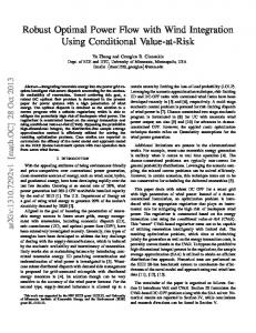
Fig. 1. Topology of the IEEE 14 bus test case with storage at each node. This figure is a modified version of the figure provided in [32]. The batteries at each node represent canonical storage units.
(6)
In (6), sk (t), the reactive part of the power flow in or out of the storage at bus k ∈ N and time t = 1, . . . , T, is limited by Skmin ≤ sk (t) ≤ Skmax .
(7)
At generation buses l ∈ G and time t = 1, . . . , T, the active power generation P lg (t) and the reactive power generation Qgl (t) are bounded as
We use the convention that P kg (t) = 0 and Qgk (t) = 0 for k ∈ N \G and t = 1, . . . , T and rk (T ) = 0 and sk (T ) = 0
Plmin ≤ Plg (t) ≤ Plmax , ≤ Qgl (t) ≤ Qmax . Qmin l l
1 With some abuse of notation r (t) denotes the energy charged/discharged k at storage at bus k over the period [t, t + 1].
(1a) (1b)
for k ∈ N . Then, given the parameters in Table II, an optimal power flow problem with storage dynamics is written as ϕ∗ := min
T � �
, one can show that the problem in (8) is equivalent to the following optimization
2
cl2 (t) (Plg (t)) + cl1 (t)Plg (t)
t=1 l∈G
ϕ∗ = (8)
subject to (1), (2), (3), (4), (5), (6), and (7)
αl (t)
(11)
t=1 l∈G
Pkmin − Pkd (t) ≤ tr {Yk W (t)} + rk (t) ≤ Pkmax − Pkd (t), � − Qdk (t) ≤ tr Yk W (t) + sk (t) Qmin k
(12a)
≤ Qmax − Qdk (t), k min 2 ≤ tr {Mk W (t)} ≤ (Vkmax )2 , Vk
(12b)
0 ≤ bk (t) ≤ Bkmax , min Rk ≤ rk (t) ≤ Rkmax , Skmin ≤ sk (t) ≤ Skmax ,
(12d) (12e)
�
bk (t + 1) = rk (t) + bk (t), �
III. S OLUTION STRATEGY The problem in (8) is nonconvex in general (e.g., due to the nonconvexity of the constraint (2) and the bilinearity in the equality constraint in (6)). We now propose a convex relaxation of (8) and show that, under certain conditions, a solution to (8) can be constructed from that for this relaxation. To this end, we follow a similar procedure discussed in [22], [23] and partly adopt their notation. A. Reformulation of the OPF problem with storage Let ek ∈ Rn , k = 1, . . . , n, be the standard basis vectors for Rn and define � � ek e∗k 0 Mk := , 0 ek e∗k Yk := ek e∗k Y, � � � � � � 1 Re �Yk + YkT � Im �YkT − Yk � Yk : = , Re Yk + YkT 2 Im Yk − YkT � � � � � � 1 Im �Yk + YkT � Re �Yk − YkT � Yk : = − , Im Yk + YkT 2 Re YkT − Yk � � Re(V (t)) U (t) := , Im(V (t)) where Re(·) and Im(·) denote the real and imaginary parts of their arguments, respectively. Note that � � Re{Vk (t)Ik∗ (t)} = tr Yk U (t)U T (t) , (9a) � � ∗ T Im{Vk (t)Ik (t)} = tr Yk U (t)U (t) , (9b) � � |Vk (t)|2 = tr Mk U (t)U T (t) , (9c) where tr(·) denotes the trace of its argument. By substituting Pkg (t) = Re{Vk (t)Ik∗ (t)} + Pkd (t) + rk (t)
(10a)
Qgk (t) = Im{Vk (t)Ik∗ (t)} + Qdk (t) + sk (t)
(10b)
W (t) := U (t)U (t)T
W (t),α(t),b(t),r(t),s(t)
T � �
subject to
over the decision variables V k (t), Pkg (t), Qgk (t), bk (t), rk (t), and sk (t) (with the index k and time t running over the sets according to the description above). Note that, in the conventional OPF formulation without storage, there is no correlation across time; therefore, the corresponding optimization is static and can be solved independently at each time. The admittance matrix induces optimization across the different generators. Storage allows optimization across time, i.e., charge when the cost of generation is low and discharge when it is high.
for Pkg (t), Qgk (t) and then defining
min
(12c)
(12f) (12g)
bk (1) = gk , � al0 (t) al1 (t) � 0, al1 (t) −1 W (t) � 0,
(12h)
rank(W (t)) = 1,
(12k)
(12i) (12j)
where
� � al0 (t) := cl1 (t) tr {Yl W (t)} + rl (t) + Pld (t) − αl (t), � � � al1 (t) := cl2 (t) tr {Yl W (t)} + rl (t) + Pld (t) .
For symmetric matrix X, X � 0 (X � 0) means that X is positive (negative) semi-definite. As before, in (11)-(12), k ∈ N , l ∈ G and the time index t = 1, . . . , T except for (12g) where t runs over {1, . . . , T − 1}. Also P kg (t) = 0 and Qgk (t) = 0 for k ∈ N \G and t = 1, . . . , T with rk (T ) = 0 and sk (T ) = 0 for k ∈ N . Note that the constraint in (12i) 2 is equivalent to cl2 (t) (Plg (t)) + cl1 (t)Plg (t) ≤ αl (t) by the substitution in (10) and the Schur complement formula [7]. The equivalence between (8) and (11)-(12) follows from the fact that a symmetric matrix X ∈ R n×n is positive semidefinite and of rank 1 if and only if there exists x ∈ R n such that X = xxT . Finally, note that the optimization in (11)-(12) has a linear cost function along with convex constraints (linear equality and inequality constraints in (12a)-(12h) and linear matrix inequalities in (12i)-(12j)) and a single nonconvex constraint in (12k). B. Lagrangian relaxation for the OPF problem with storage We now develop a Lagrangian dual for optimization (11)(12) excluding the nonconvex rank constraints in (12k). To this end, let us introduce zl (t) := [zl0 (t), zl1 (t), zl2 (t)]T ,
l ∈ G, t ∈ {1, . . . , T },
and
� x(t) := λmin (t)T , λmax (t)T , η min (t)T , η max (t)T , μmin (t)T , μmax (t)T , γ min (t)T , γ max (t)T , �T ρmin (t)T , ρmax (t)T , ξ min (t)T , ξ max (t)T ,
and define h(x, z, σ, β) := − +
T � �
zl2 (t) −
t=1 l∈G T � �
�
βk g k
k∈N
�
Λk (t)Pkd (t) + Hk (t)Qdk (t)
t=1 k∈N
+ λmin (t)Pkmin − λmax (t)Pkmax k k + ηkmin (t)Qmin − ηkmax (t)Qmax k k
2 min 2 max + μmin (t) V − μ (t) (Vkmax ) k k k + ρmin (t)Rkmin − ρmax (t)Rkmax k k − γkmax (t)Bkmax
� + ξkmin (t)Skmin − ξkmax (t)Skmax , where
⎧ max min ⎪ ⎨ λk (t) − λk (t) � Λk (t) := +ck1 (t) + 2 ck2 (t)zk1 (t), ⎪ ⎩ max λk (t) − λmin (t), k ∈ N \G, k
Hk (t) := ηkmax (t) − ηkmin (t),
k ∈ N,
Υk (t) := μmax (t) − μmin (t), k k
k∈N
k ∈ G,
λmax (t) = 1, k ηkmax (t) = ηkmin (t) = 1,
Consider the optimization
subject to ��
correspond to (12i) and Ω(t) � 0 correspond to (12j). Then, by standard manipulations on the Lagrangian for optimization (11)-(12) (with the dual variables defined above), showing that zl0 (t) = 1 (through minimization of the Lagrangian with respect to αl (t)), and eliminating Ω(t), optimization (13)-(14) is a Lagrangian dual of that in (11)-(12) excluding the rank constraint in (12k). To show that strong duality holds, note that both optimization problems (13)-(14) and (11)-(12) excluding the rank constraint in (12k) are convex. A strictly feasible solution can be constructed as � ck1 (t) + 1, for k ∈ G min λk (t) := 1, for k ∈ N \G and for k ∈ N ,
for t ∈ {0, . . . , T }. ψ ∗ :=
where, in each case, the variable with the superscript “max” (“min”) corresponds to the upper (lower) bounds and the indices k and t run over the sets as indicated in (12). For k ∈ N and t = 1, . . . , T − 1, σk (t + 1) corresponds to the constraint bk (t + 1) = bk (t) + rk (t) in (12g), and β k corresponds to that in (12h). Finally, let � � zl0 (t) zl1 (t) �0 zl1 (t) zl2 (t)
max h(x, z, σ, β)
(t) = 2, μmax k
(13)
x�0,z,σ,β
μmin (t) = 1, k � Λk (t)Yk + Hk (t)Y k + Υk (t)Mk � 0,
(14a)
k∈N
Hk (t) + ξkmax (t) − ξkmin (t) Λk (t) + ρmax (t) − ρmin (t) + σk (t + 1) k k σk (t + 1) − σk (t) + γkmax (t) − γkmin (t) σk (2) + γkmax (1) − γkmin (1) + βk −σk (T ) + γkmax (T ) − γkmin (T ) �
1 zl1 (t) zl1 (t) zl2 (t)
�
= 0,
(14b)
= 0,
(14c)
= 0,
(14d)
= 0,
(14e)
= 0,
(14f)
� 0,
(14g)
where the indices k run over N and l over G. The time index t = 1, . . . , T in (14a), (14b) and (14g), t = 1, . . . , T − 1 in (14c), and t = 2, . . . , T − 1 in (14c)-(14d). Theorem 1: Optimization (13)-(14) is a Lagrangian dual of optimization (11)-(12) excluding the rank constraints in (12k) and strong duality holds. Proof: Introduce the following correspondence between the constraints in (12) (all constraints on reals written as f (y) ≤ 0 with f : Rν → R and all constraints on symmetric matrices written as f (y) � 0 with f : Rν → Rω×ω ) and the decision variables in (13)-(14) as λmax (t), λmin (t) ≥ 0 k k max ηk (t), ηkmin (t) ≥ 0 μmax (t), μmin (t) ≥ 0 k k max γk (t), γkmin (t) ≥ 0 ρmax (t), ρmin (t) ≥ 0 k k max ξk (t), ξkmin (t) ≥ 0
for (12a), for (12b), for (12c), for (12d), for (12e), for (12f),
(t) = ρmin (t) = 1, ρmax k k γkmax (t) = γkmin (t) = 1 ξkmax (t) = ξkmin (t) = 1, and βk = 0, where the time indices take values in {0, . . . , T } along with zl0 (t) = 0, zl1 (t) = 1 for l ∈ G and t ∈ {0, . . . , T }, σk (t+1) = 0 for k ∈ N with time taking values in {0, . . . , T −1}. Hence, strong duality holds by Slater’s theorem [7]. C. Constructing an optimal solution for OPF with storage Theorem 1 shows that there is no duality gap between optimization (13)-(14) and the rank relaxation in (11)-(12) of the (equivalent) reformulation of the OPF problem with storage. In this section, we show, under certain assumptions, that there is no duality gap between the optimizations in (13)(14) and (11)-(12). Assumptions: 1) Optimization (11)-(12) is feasible and every feasible solution satisfies W (t) �= 0 for all t ∈ {1, . . . , T }. 2) There exists an optimal solution to (13)-(14) with optimal values (xopt (t), z opt (t)) for (x(t), z(t)) such that � � opt � Aopt (t) := Λk (t)Yk + Hkopt (t)Y k + Υopt k (t)Mk k∈N
has a zero eigenvalue of multiplicity two for t = 1, . . . , T.
Remark 1: Assumption 1 is to avoid trivial solutions and implies that V (t) = 0 is not feasible for (11)-(12) and equivalently for (8) for any t. Remark 2: Assumption 2 is critical (as discussed in the following) for constructing a solution to the problem in (11)-(12) from that in (13)-(14) (through the KKT condition tr(W opt (t)Aopt (t)) = 0 for each t = 1, . . . , T ). Note that Assumption 2 can only be verified once the problem in (13)(14) has been solved. Moreover, it limits the instances of the problem in (11)-(12) for which a solution can be constructed. On the other hand, references [22], [23] discuss algebraic and geometric interpretations of Assumption 2 under the extra condition that Y is symmetric with nonnegative offdiagonal entries in Re(Y ) and nonpositive off-diagonal entries in Im(Y ). Theorem 2: Under Assumptions 1 and 2, ϕ ∗ = ψ ∗ and an optimal solution to (11)-(12) (and equivalently for (8)) can be constructed from the solution of (13)-(14). The proof of Theorem 2 is a straightforward extension of a similar result in the case with no storage in [22, Theorem 1]. Summary of the resulting computational procedure: We now summarize how the results of this section can be used to compute a solution to the OPF problem with storage in (8). The procedure is based on solving the problem in (13)-(14) instead of that in (8). If the problem (13)-(14) is feasible and the solution satisfies Assumption 2, then the computational procedure for constructing the optimal solution to the OPF problem with storage (8) is as follows: Let [ν 1 (t)T ν2 (t)T ]T be in the null space of A opt (t) with ν1 (t), ν2 (t) ∈ Rn . Then, an optimal value V opt (t) for V (t) can be computed as V opt (t) = (ζ1 (t) + ζ2 (t)i)(ν1 (t) + ν2 (t)i), where the constants ζ1 (t) and ζ2 (t) can be determined from the KKT conditions μmin (t)((Vkmin )2 − |Vk (t)|2 ) = 0, k (t)(|Vk (t)|2 − (Vkmax )2 ) = 0 μmax k and the fact that the phase angle at the swing (reference) bus is known (e.g., zero). An optimal value of W (t) can be computed through W (t) = U (t)U (t) T . Then, optimal values for P g , Qg , b, r, and s are computed through the KKT conditions: for k ∈ N , � � (t) tr{Yk W (t)} + rk (t) − Pkmin + Pkd (t) = 0, λmin k � � λmax (t) Pkmax − Pkd (t) − tr{Yk W (t)} − rk (t) = 0, k � � ηkmin (t) tr{Yk W (t)} + sk (t) − Qmin + Qdk (t) = 0, k � � ηkmax (t) Qmax − Qdk (t) − tr{Yk W (t)} − sk (t) = 0, k γkmin (t)bk (t) = 0,
γkmax (t) [Bkmax − bk (t)] = 0,
for t = 1, . . . , T, � � (t) rk (t) − Rkmin = 0, ρmin k � � ξkmin (t) sk (t) − Skmin = 0,
ρmax (t) [Rkmax − rk (t)] = 0, k ξkmax (t) [Skmax − sk (t)] = 0,
σk (t + 1) [rk (t) − bk (t + 1) + bk (t)] = 0, for t = 1, . . . , T − 1, and βk [bk (1) − gk ] = 0 and the conditions in (10). Note that the KKT conditions constitute
a set of affine equality constraints on the decision variables P g , Qg , b, r, and s. If the optimal value of the optimization in (13)-(14) is unbounded, the problem in (8) is infeasible (because the rank relaxation of the equivalent reformulation in (11)-(12) is infeasible). If the problem in (13)-(14) is feasible but its solution violates Assumption 2, the procedure is inconclusive (i.e., a solution for the optimization in (8) cannot be constructed). IV. C ASE STUDIES In this section, we illustrate the effect of energy storage using the IEEE 14 bus benchmark example [32] with different cost functions of the form (8) by using the computational procedure discussed in the previous section. This benchmark system, which represents a portion of the Midwestern US Electric Power System as of February, 1962 [32], does not include storage. Therefore, while we use its network topology as well as its voltage and generation bounds, (i.e., V max , V min , P max , P min , Qmax and Qmin in (1) and (2)), we need to add appropriate values for the storage parameters as well as time-varying demand profiles. We created demand profiles for each bus using typical hourly demands for 14 different 2009 December days in Long Beach, CA, USA [1]. The curves are scaled so that their peak corresponds to the static demand values in the IEEE 14 bus test case. Figure 2(a) shows the demand curves for each bus. For all of the results presented here the rate limits in Mega Watts (MW) (5) are set to be between 25 − 33% of the maximum capacity of the storage, e.g. 0.25BmaxΔt with Δt = 1. The limits Skmax and Skmin in (7) on the reactive power are set to keep the rate angle between −18 deg and 48 deg. This range was selected based on the real and reactive generation limits in the IEEE 14 bus test case which give rise to generator angles approximately between −17 deg and 90 deg. Unless otherwise indicated all power values reported in the following sections are normalized to per unit values (p.u.) as described in [24]. A. Example I: Linear cost We first use a cost function that is the sum of the total � � generation (i.e., P g 1 = Tt=1 l∈G Plg (t)) and refer to this as a time-invariant linear cost function since the coefficients cl1 (t) = 1 and cl2 (t) = 0 from (8) are constant in time for each l ∈ G. Figure 2(b) shows that the addition of storage (32 MWh per bus) as well as the finite-horizon optimization produces a flatter generation curve over the time period. This change is most evident for generators 4 and 5 (respectively P4g and P5g ). For this cost function, the optimal solution did not make use of generator 1. A constant generation profile is desirable from an operator perspective as the efficiency of most of the conventional generators are optimized for full capacity. As a result, many operators maintain generation levels that will accommodate the peak demand which can lead to excess power being curtailed. There has been a great deal of research aimed at demandbased pricing strategies, (i.e., higher prices at peak demand times). In order �T to�simulate thisg effect we use a weighted � 1 norm (i.e., l∈G cl1 (t)Pl (t)) for the cost function in t=1
1 Load buses Generator Buses
0.9
P2g (p.u.)
P1g (p.u.)
0.24 0.04 0.02 0
0.2 0.16 0.12 0.08
0.8
1
P d (p.u.)
0.6 0.5
0.5
P4g (p.u.)
P3g (p.u.)
0.7
0.8 0.6 0.4 0.3
0.4
0.4 0.3 0.2 0.15
1
1
4
8
P5g (p.u.)
0.2 0.1 0
1
4
8
12
16
20
16
20
24
0.8 No storage storage, time−invariant cost storage, time−varying cost
0.6 0.4
24
12
Time (hours)
0.3
1
4
Time (hours)
8
12
16
20
24
Time (hours)
(a)
(b)
Fig. 2. (a) Hourly demand peak scaled to match the demands in IEEE 14 bus benchmark case. The load profiles represent demands for 14 different typical days in December 2009 in Long Beach, CA, USA. (b) Hourly generation for each l ∈ G. The addition of 32 MWh storage at each bus as well as optimization over time results in flatter generation profiles, especially when a demand-based time-varying cost function is used. This smoothing of the generation curve is most evident for generators 4 and 5, with this cost function generators 2 and 3 produce power primarily to track their own load.
0.2
P2g (p.u.)
P1g (p.u.)
0.04
0.02
0.15
0
2.6
Total Demand
0.1
2.4
Total Generation 6 MWh per bus
0.8
0.6
0.4 0.3 0.2
0.4
1
P5g (p.u.)
1
4
8
12
16
20
24
Time (hours)
0.8
Total Generation 12 MWh per bus
2.2
Total Generation 32 MWh per bus 2 1.8 1.6 1.4
No storage storage, 6 MWh per bus storage, 12 MWh per bus storage, 32 MWh per bus
0.6 0.4
Total Power (p.u)
P4g (p.u.)
P3g (p.u.)
1
1
4
8
12
16
20
24
Time (hours)
1.2 1
1
4
8
12
16
20
24
Time (hours) (a)
(b)
Fig. 3. (a) Hourly generation for each l ∈ G given a demand-based time-varying linear cost function over a range of per-bus storage levels. Increasing the level of per-bus storage increases the amount of reduction in generation peaks but even low levels of storage effectively shave the peak. Note that the increase in benefits with increasing storage does not continue indefinitely as is shown through the saturation in Figure 5(a) . For all storage levels this smoothing of the generation curve is most evident for generators 4 and 5 and generators 2 and 3 continue produce power primarily to track their own load.
(8) where for each generator l ∈ G the parameter c l1 (t) = 1 for t ∈ {1, . . . 15} and cl1 (t) = 1.5 for t ∈ {16, . . . 24} and refer to this case as the time-varying cost function (where t = 15 corresponds roughly to the time at which the demand values in Figure 2(a) begin to increase). Figure 2(b) shows that such a time-varying cost function further regulates the demand profile to an essentially constant level for generators 4 and 5 and reduces the peak-to-trough spread on generator 2. Some of the demand is also supplied by requiring a small amount of generation from generator 1 during the peak period. It should be noted that generators 2 and 3 produce power primarily to track their own load, for both the time-invariant
and time-varying linear cost functions. One reason that the finite-horizon optimization with storage does not flatten all of the generation profiles is because the linear cost function (i.e., �1 norm based) only attempts to minimize overall generation rather than the total energy of the power signal. Figure 3(a) shows the results of using time-varying linear cost function at two additional storage levels. The reduction in the generation peak begins with storage levels as low as 6 MWh per bus, which corresponds to a storage capacity that can handle 2% of the full daily demand or 33% of the peak load. It should be noted the optimal solution computed for this case study favors storage at only the non-generating nodes.
Demand (p.u.)
0.5
0
1.06
|V | (Volts)
Demand (p.u.) |V | (Volts)
1
1.04 1.02
1
0.5
0
1.06 1.04 1.02
�
V (radians)
0.1 0 −0.1 −0.2
0.1 0 −0.1
�
V (radians)
0.2 0.2
−0.2 1
4
8
12
16
20
24
1
4
8
Node 1
Node 2
Node 3
12
16
20
24
Time (hours)
Time (hours) Node 6
Node 8
(a)
Node 1
Node 2
Node 3
Node 6
Node 8
(b)
Fig. 4. The variation in voltage magnitude and angle for l ∈ G (i.e., at the generator nodes) over time. The top panels both in (a) and (b) show the demand in p.u., the middle panels show the voltage magnitude |V | in p.u. and the bottom panels show the corresponding angle ∠V for (a) the per-bus storage capacity is B max = 6 MWh and in (b) the per-bus storage capacity is Bmax = 12 MWh. For both cases, the cost function is linear and time-varying.
Therefore, the actual storage use represents 1.4% of the system capacity or 21% of the peak load. The reason that the storage use is distributed in this manner and the general problem of optimal storage placement is a topic of ongoing study [29]. As expected the amount of benefit from the storage increases with the storage capacity. The benefit of the added storage capacity in reducing the overall system load is illustrated in Figure 3(b), which shows the aggregated system demand and generation for 6, 12 and 32 MWh of storage per bus using the same time-varying linear cost function. The addition of storage results in 5.7% and 10% peak reductions for 6, 12 MWh of per-bus storage capacity. Figure 4 shows the changes in voltage magnitude and angle at the generator nodes as a function of time for 6 and 12 MWh of per-bus storage capacity. The top panels of each figure shows the corresponding demand curves whereas the middle and bottom panels respectively show the voltage magnitude |V | in p.u. and angle ∠V at each time. In most cases, the nodes with the highest demands correspond to the lowest voltage variations whereas the nodes with the low demand correspond to the higher voltage variations. In contrast the largest angle changes occur at the nodes with the lowest demands. These trends are expected because a high power draw is likely to cause a drop in voltage. Comparing the voltage levels on figures 4(a) and 4(b), the increased storage provides some smoothing of the voltage magnitudes especially through the peak period. This trend is most obvious from t = 17 . . . 23 where nodes 1, 2, 3 and 6 show much smoother voltage curves for the higher storage capacity case (Figure 4(b)). Figure 5(a) shows how the value of both time-invariant and time-varying cost functions (normalized such that each Plg (t) for l ∈ G and t ∈ {0, . . . T } is a p.u. value) change with the amount of per-bus storage capacity B kmax in MWh. For the time-independent cost function (which is equivalent to
total generation), the storage reduces the cost by only a small percentage. While, the addition of a simple demand-based cost structure increases the cost benefit of adding storage by about 0.8% for every 8 MWh of per-bus storage capacity that is added to the system. B. Example II: Quadratic cost In this subsection, we repeat the computations described in section IV-A for both time-invariant and time-varying quadratic cost functions. Again, we use the peak normalized demand profiles shown in the top panel of Figure 7(a) to determine that t = 15 is the time step where the average demand starts to increase toward peak levels. The higher cost function coefficients for t ≥ 15 are thus meant to reflect a demand-based pricing scheme. We obtain the second-order coefficients directly from the IEEE 14 bus test case. The linear coefficients were selected to maintain the ratio of costs between the generators in the test case. For the time-invariant case the coefficients for t = 1, . . . , 24, are c 12 (t) = 0.043, c22 (t) = 0.250, cl2 = 0.01 for l = 3, 4, 5, cl1 (t) = 2 for l = 1, 2, and cl1 (t) = 4 and cl2 (t) = 0.010 for l = 3, 4, 5. For the time-varying case the quadratic term coefficients, c l2 (t) for l ∈ {1, . . . , 5} and for all t, are the same as in the timeindependent case. The first-order coefficients c l1 (t) = 2 for l = 1, 2 and cl1 (t) = 4 for l = 3, 4, 5 for t = 1, . . . , 15, and cl1 (t) = 4 for l = 1, 2 and cl1 (t) = 8 for l = 3, 4, 5 for t = 16, . . . , 24. Figure 5(b) indicates that the addition of storage visibly reduces the cost function even with a time-independent cost function coefficients. The reduction is roughly 0.3 for the first 8 MWh of per-bus storage capacity and then the added savings with increasing amounts of storage drops off rapidly especially at storage capacities greater than 32 MWh per bus. As with the linear cost function, the value for the time-varying case decreases approximately linearly with increasing storage but the slope is significantly steeper. In
0.9
Cost function (normalized)
0.995
P d (p.u.)
1 time−varying costs fixed costs
0.99
0.8 0.7 0.6 0.5 0.4
0.985
0.3
0.98 32
Storage (MWh)
0.975 0.97 0.965 0.96 0.955
20
10
0
0
10
20
30
Bkmax
40
50
60
70
72
(MWh per bus)
Storage (MWh)
0.95
1 0.98
60
40
20
0 1
time−varying costs fixed costs
0.96
4
8
12
16
20
24
Time (hours)
0.94
(a)
0.92
1.8
0.9
Total storage capacity
1.6 0.88
Storage capacity 1.4
at load−only buses
0.86 0.84
0
10
20
30
40
50
60
70
80
B max (MWh per bus)
(b) Fig. 5. Cost versus per-bus storage capacity (Bmax in MWh) at each bus. (a) Linear cost function. (b) Quadratic cost function. The cost always decreases with increased storage capacity. For time-varying coefficients the decrease in cost is roughly linear as a function of per-bus storage capacity for both cost functions.
Storage Use (p.u.)
Quadratic cost function (normalized)
(a)
1.2 1 0.8 0.6 0.4 0.2 0 −0.2
1
4
8
12
16
20
24
Time (hours)
(b) Fig. 7. (a) The top panel shows the peak normalized demand. At t = 15, the average demand (shown as the thick dashed-line and excluding buses with no demand) starts to increase toward peak levels, this defines the point where the cost function coefficients are increased to reflect a demand-based pricing scheme. The center and lower panels respectively show the storage use for the time-varying quadratic cost function based on per-bus capacity constraints of 32 and 72 MWh respectively. For the higher storage capacity, the full capacity is not used at any of the nodes. (b) Illustration of total system storage used versus storage capacity for the full system and the load-only nodes for the case Bmax = 12 MWh at each bus.
2
P1g (p.u.)
1.8 1.6 1.4 1.2 1 0.8
P2g (p.u.)
0.8
0.6
0.4
0.2
1
4
8
12
16
20
24
Time (hours) 32 MWh per bus
12 MWh per bus
No storage
Fig. 6. Generation comparison for storage (with Bmax = 12 and Bmax = 32 MWh per bus) and no storage with quadratic time-varying cost functions. Generators 3–5 do not generate power for either scenario.
this case, each additional 8 MWh of per-bus storage capacity storage reduces the cost function value by roughly 2% until we reach a limit beyond which additional storage no longer affects the cost function value (approximately when there is 64 MWh available at each bus). Figure 6 shows that a quadratic time-varying cost function along with storage further flattens the generation profiles and this effect increases as the per-bus capacity is increased. For the quadratic time-varying costs, generators 1 and 2 provide all of the required power. Clearly, the form of the cost function favors the use of the first two generators. The addition of
storage and an optimization over time produce almost constant levels of generation for generator 1 over the 24 hour period when compared to the no-storage case. At the highest storage capacity 32 MWh per bus the power range for generator 2 is reduced from [0.24, 0.71] to [0.30, 0.54]. Figure 7(a) shows the relationship between storage use and demand for the time-varying quadratic cost function. The top panel reflects peak normalized demand at each bus. The average per-bus demand (excluding buses with no demand) is superimposed on the rest of the curves with a thick dashedline. The center and lower panels reflect the storage use with two different per-bus capacity constraints (respectively, B max = 32 MWh and B max = 72 MWh). As the demand increases, the storage is charged until the time increment before the first local peak (at t = 8), then the storage is used to reduce the generation load until the demand stabilizes. Finally, the storage is recharged until the peak load, and then discharged until the end of the day. For the higher storage capacity constraint (B max = 72 MWh) the storage is never fully charged. The maximum usage occurs at approximately 64 MWh, which explains why the cost function value does not change for the last two points (per-bus B max levels) on Figure 5(b). As discussed in Section IV-A the optimal solution results in the use of storage only at the non-generating nodes which means that some of the capacity is not being used. This fact is illustrated using Figure 7(b), which shows the aggregate system storage use for the case of B max = 12 MWh per bus with the full system and load-only node aggregate capacities indicated. Similar results hold for all of the storage capacities that were studied and this phenomena is being investigated as part of a larger ongoing study related to optimal storage placement. Remark 3: It was observed in [22] that Assumption 2 in section III-C is satisfied in many of the IEEE benchmark systems when a small amount of resistance (e.g., of the order of 10 −5 per unit) was added to each transformer. In the numerical examples in this paper, we implement this modification. This modification essentially renders the graph induced by Re(Y ) strongly connected. V. S UMMARY AND POTENTIAL EXTENSIONS We formulated an optimal power flow problem with simple charge/discharge dynamics for energy storage collocated with load and/or generation buses as a finite-time optimal control problem. The resulting optimization problem, under certain conditions (discussed in the previous sections), was solved using a procedure based on a convex semi-definite program obtained as a Lagrangian dual to the rank relaxation of an equivalent formulations for the OPF problem with storage dynamics. We investigated effects of storage capacity and power rating on generation costs and peak reductions using a modified version of the IEEE 14 benchmark system which represents a portion of the Midwestern U.S. Electric Power System. As discussed in the earlier sections, the motivation of the current work is to assess the utility of grid-integrated storage
in mitigating issues associated with integration of intermittent renewable energy resources into the electric power grid. As a step toward this goal, the current paper investigated only the impact of the large scale integration of energy storage. Integration of uncertainties due to either intermittency in generation or fluctuations in demand is a subject of ongoing study (with preliminary work reported in [29]). Another natural extension is assessing effects of the distribution of energy storage systems in the power grid to minimize losses and defer the expansion requirements of transmission capacities. The role of energy storage is to provide flexibility to the power systems for dealing with a number of concerns including power quality, stability, load following, peak reduction, and reliability. A promising direction is assessing the suitability of hybrid storage technologies (e.g., a combination of pumped-hydro, thermal, and batteries) in addressing these issues. Additionally, similar flexibility can be acquired through spinning reserves and/or conventional generators with high ramp rates. An interesting design issue is deciding on an appropriate balance between the storage and ancillary generation capacities. ACKNOWLEDGEMENTS The authors gratefully acknowledge George Rodriguez and Christopher Clarke of Southern California Edison as well as Mani Chandy of the California Institute of Technology for fruitful discussions and helpful suggestions. R EFERENCES [1] Personal communication with researchers from Southern California Edison. [2] T. Ackerman, Ed., Wind Power in Power Systems. Wiley, 2005. [3] N. Alguacil and A. J. Conejo, “Multiperiod optimal power flow using benders decomposition,” IEEE Trans. Power Systems, vol. 15, no. 1, pp. 196 –201, 2000. [4] Y. M. Atwa and E. F. El-Saadany, “Optimal allocation of ESS in distribution systems with a high penetration of wind energy,” IEEE Trans. on Power Systems, vol. 25, no. 4, pp. 1815–1822, Nov. 2010. [5] X. Bai, H. Wei, K. Fujisawa, and Y. Wang, “Semidefinite programming for optimal power flow problems,” Int’l J. of Electrical Power & Energy Systems, vol. 30, no. 6-7, pp. 383–392, 2008. [6] J. P. Barton and D. G. Infield, “Energy storage and its use with intermittent renewable energy,” IEEE Trans. Energy Conversion, vol. 19, no. 2, pp. 441–448, 2004. [7] S. Boyd and L. Vandenberghe, Convex Optimization. Cambridge Univ. Press, 2004. [8] V. Budhraja, F. Mobasheri, M. Cheng, J. Dyer, E. Castano, S. Hess, and J. Eto, “California’s electricity generation and transmission interconnection needs under alternative scenarios,” California Energy Commission, Tech. Rep., 2004. [9] J. Carpentier, “Contribution to the economic dispatch problem,” Bulletin de la Societe Francoise des Electriciens, vol. 3, no. 8, pp. 431–447, 1962, in French. [10] J. Carrasco, L. Franquelo, J. Bialasiewicz, E. Galv´an, R. P. Guisado, M. M. Prats, J. Le´on, and N. Moreno-Alfonso, “Power-electronic systems for the grid integration of renewable energy sources: A survey,” IEEE Trans. Industrial Electronics, vol. 53, no. 4, pp. 1002–1016, 2006. [11] M. Chandy, S. Low, U. Topcu, and H. Xu, “A simple optimal power flow model with energy storage,” in Proc. of Conf. on Decision and Control, 2010. [12] H. P. Chao and S. Peck, “A market mechanism for electric power transmission,” J. of Regulatory Economics, vol. 10, pp. 25–59, 1996. [13] H. P. Chao, S. Peck, S. Oren, and R. Wilson, “Flow-based transmission rights and congestion management,” The Electricity J., vol. 13, no. 8, pp. 38–58, 2000.
[14] M. Geidl and G. Andersson, “A modeling and optimization approach for multiple energy carrier power flow,” in Proc. of IEEE PES PowerTech, 2005. [15] I. P. Gyuk, “EPRI-DOE handbook of energy storage for transmission and distribution applications,” EPRI-DOE, Washington, DC, Tech. Rep., December 2003. [16] K. Heussen, S. Koch, A. Ulbig, and G. Andersson, “Energy Storage in Power System Operation : The Power Nodes Modeling Framework,” in IEEE PES Conference on Innovative Smart Grid Technologies Europe. IEEE, 2010, pp. 1–8. [17] W. W. Hogan, “Contract networks for electric power transmission,” J. of Regulatory Economics, vol. 4, no. 3, pp. 211–42, 1992. [18] M. Huneault and F. D. Galiana, “A survey of the optimal power flow literature,” IEEE Trans. on Power Systems, vol. 6, no. 2, pp. 762–770, 1991. [19] R. Jabr, “Radial Distribution Load Flow Using Conic Programming,” IEEE Trans. on Power Systems, vol. 21, no. 3, pp. 1458–1459, Aug 2006. [20] ——, “Optimal Power Flow Using an Extended Conic Quadratic Formulation,” IEEE Trans. on Power Systems, vol. 23, no. 3, pp. 1000–1008, Aug 2008. [21] J. Lavaei, “Zero duality gap for classical OPF problem convexifies fundamental nonlinear power problems,” in Proc.of the American Control Conf., 2011. [22] J. Lavaei and S. Low, “Convexification of optimal power flow problem,” in Proc. Allerton Conf. on Communication, Control and Computing, 2010. [23] ——, “Zero duality gap in optimal power flow problem,” IEEE Trans. on Power Systems, To Appear, 2011. [24] J. A. Momoh, Electric Power System Applications of Optimization, ser. Power Engineering, H. L. Willis, Ed. Markel Dekker Inc.: New York, USA, 2001. [25] J. A. Momoh, M. E. El-Hawary, and R. Adapa, “A review of selected optimal power flow literature to 1993. Part I: Nonlinear and quadratic programming approaches,” IEEE Trans. on Power Systems, vol. 14, no. 1, pp. 96–104, 1999. [26] K. S. Pandya and S. K. Joshi, “A survey of optimal power flow methods,” J. of Theoretical and Applied Information Technology, vol. 4, no. 5, pp. 450–458, 2008. [27] R. Schainker, “Executive overview: Energy storage options for a sustainable energy future,” in Proc. of IEEE PES General Meeting, 2004, pp. 2309–2314. [28] S. M. Schoenung, J. M. Eyer, J. J. Iannucci, and S. A. Horgan, “Energy storage for a competitive power market,” Ann. Rev. of Energy and the Environment, vol. 21, no. 1, pp. 347–370, 1996. [29] A. E. Sj¨odin, D. Gayme, and U. Topcu, “Risk-mitigated OPF with high wind penetration,” 2011, in prep. [30] E. Sortomme and M. A. El-Sharkawi, “Optimal power flow for a system of microgrids with controllable loads and battery storage,” in Power Systems Conf. and Exposition, 2009. [31] J. W. Tester, E. M. Drake, M. J. Driscoll, M. W. Golay, and W. A. Peters, Sustainable Energy: Choosing Among Options. MIT Press, 2005. [32] University of Washington, “Power systems test case archive.” [Online]. Available: http://www.ee.washington.edu/research/pstca/ [33] U.S. Energy Information Administration, “Annual energy outlooks 2010 with projections to 2035,” U.S. Department of Energy, Tech. Rep. DOE/EIA-0383, 2010. [Online]. Available: http://www.eia.doe.gov/oiaf/aeo [34] P. Vytelingum, T. D. Voice, S. D. Ramchurn, A. Rogers, and N. R. Jennings, “Agent-based Micro-Storage Management for the Smart Grid,” in The Ninth International Conference on Autonomous Agents and Multiagent System, Toronto, May 2010, pp. 39–46. [35] H. Xu, U. Topcu, S. Low, and M. Chandy, “On load-shedding probabilities of power systems with renewable power generation and energy storage,” in Proc. Allerton Conf. on Communication, Control and Computing, 2010. [36] T. Yau, L. Walker, H. Graham, and A. Gupta, “Effects of battery storage devices on power system dispatch,” IEEE Trans. Power Apparatus and Systems, vol. PAS-100, no. 1, pp. 375–383, 1981. [37] R. D. Zimmerman, C. E. Murillo-S´anchez, and R. J. Thomas, “MATPOWER’s extensible optimal power flow architecture,” in Proc. IEEE PES General Meeting, 2009, pp. 1–7.