Distributed Real-Time Power Flow Control with Renewable Integration Kiyoshi Nakayama∗ , Changhong Zhao† , Lubomir F. Bic∗ , Michael B. Dillencourt∗ , Jack Brouwer‡ ∗
Dept. of Computer Science, University of California, Irvine, CA 92697-3435, USA Dept. of Electrical Engineering, California Institute of Technology, Pasadena, CA 91125-0001, USA ‡ Dept. of Mechanical and Aerospace Engineering, University of California, Irvine, CA 92697-3550, USA Email:
[email protected],
[email protected], {bic, dillenco}@ics.uci.edu,
[email protected] †
Abstract—We formulate an Optimal Real-Time Power Flow (ORPF) problem that integrates renwable energy generation and energy storage. In the ORPF problem, we seek to minimize the costs of energy storage and of power generation from fossil fuel that are required to balance the loads and generation from renewable sources. We present a novel decentralized algorithm for this problem, using tie-set graph theory. Tie-set graph theory significantly reduces the complexity of the ORPF problem by dividing a power network into a set of independent loops referred to as “tie-sets.” Simulation results demonstrate real-time power production responses and flow controls that lead to reliable use of battery systems and reduce the cost of using fossil fuel.
I. I NTRODUCTION Integration of renewables with energy storage systems has been motivated by the increasing availability of renewable energy from solar and wind power and excess generation by customers. According to [1], “It has been estimated that if 20% of the energy that could be harvested from wind farms across the globe were used, all of the world’s electricity demands could be met several times over [2].” Battery systems provide large savings in generation cost without compromising energy availability for customers [3]. Optimal power flow (OPF) problems, first formulated and studied by Carpentier [4], have been studied for more than half a century. Many of the earlier models for OPF focused on static optimizations, i.e., optimizations for isolated periods of time in which power supply and demand must be balanced at every period. Today, it is increasingly common for energy storage devices such as batteries to be installed and used in power grids [5]. By charging and discharging the batteries, mismatches between instantaneous power supply and demand can be balanced. As a result, the requirement of power balance at every instant in the OPF formulation can be relaxed. Multiperiod versions of OPF problems can be considered. in which the battery charging/discharging profile becomes one of the control variables over which the optimization is defined. In this paper, we adopt a model similar to that of [1]. We formulate an Optimal Real-Time Power Flow (ORPF) problem with energy storage devices. Our goal is to minimize the total cost, which consists of (1) the cost of power production by the Controllable Generation Facility (CGF) using fossil fuels and (2) the cost of using batteries across multiple time periods to balance the fluctuation of renewable power generation and loads. To solve the ORPF problem, we present a novel
decentralized algorithm to autonomously allocate the CGF generations and battery charges/discharges. As the topology of today’s traditional grids are modified to integrate and manage distributed energy resources (DERs), mesh topologies will likely be utilized because of the increased flexibility, efficiency, and resiliency they provide [6], [7]. The proposed algorithm effectively divides a meshed power network into a set of independent loops, so-called “tie-sets” in graph theory, that can be seen as a µ-dimensional linear vector space1 . Monitoring of loads and renewable production is locally conducted in each tie-set using an autonomous agent. Based on the monitored data, each tie-set independently optimizes the power production response and then distributes power flow at each time step to minimize both CGF and battery cost. The work in [8] deals with balanced allocation of static distributed energy resources and introduces the simulation results showing that the iterative optimization within the system of fundamental system of tie-sets leads to global solution whose theoretical property can be verified in [9]. On the basis of [8], our previous work achieves the balanced allocation of renewables with the complete automation of a prospective future grid that integrates end-use devices to capture stochastic process of loads and renewable generations automatically [10]. The proposed algorithms achieve sustainable grid operation even though future load is uncertain and renewable generation is variable and unpredictable. Simulation results show that our algorithm reduces the costs of battery usage and power production by CGF at every time step, and demonstrates flow distribution that leads to reliable use of battery systems. II. P ROBLEM F ORMULATION In this section, we formulate an Optimal Real-Time Power Flow (ORPF) problem that integrates renewable energy production and energy storage devices. We consider a connected graph G = (V, E) with a set of nodes V = (1, ..., n) representing the buses and a set of links E ⊆ V ×V representing the power lines. The links are directed with arbitrarily defined directions, and a link from nodes i to j is denoted interchangeably by either (i, j) ∈ E or i → j. 1 µ is the nullity of an underlying graph of a power grid as defined in Section III-A.
Let i : i → j and k : j → k denote the set of predecessors and successors of node j in the directed graph, respectively. We focus on the notion of a system operating point (SOP) [11], which has a task of integrating growing amounts of renewables as well as loads and in- and-out power flows into a smart grid. A node in this model has the function of SOP and is also responsible for making a decision to balance the supply and load at every moment, with the help of installed storage devices, e.g., batteries. Storage systems are significantly able to save generation cost without wasting consumers’ facilities, by charging or discharging to balance the surplus or shortfall in generation compared to load. Then, we define the following variables in the power network. • pj (t): The battery energy level at node j ∈ V at time t ∈ T := {1, 2, ...}. • lj (t): The total load of node j at time t. • rj (t): The amount of real power injection of node j at time t that is provided by renewable energy resources. • gj (t): The amount of real power injection of node j at time t provided from Controllable Generation Facility (CGF) that utilizes resources except renewable resources, such as fossil fuel (coal, gas powered) or nuclear. • fij (t): The real power flow on the link (i, j) ∈ E. We use variables without subscripts to denote vectors with the proper components. For example, p = (pj (t), j ∈ V and t ∈ T ) denotes the vector of node battery energy levels. The battery energy levels pj follow the dynamics as 2
ORPF: Given initial battery levels p(0) ≥ 0, net demand d, battery capacities p, CGF capacities g, link capacities f , and a given time sequence T = {t}, the ORPF is ∑ ∑( ) min ci (gi (t), t) + bi (pi (t)) (6)
pj (t) = pj (t − 1) − dj (t) + gj (t) − Fj (t), for j ∈ V, (1)
Tie-set graph theory is described in detail in [12], [13]. Here we provide the basics. For a given bi-connected graph G = (V, E), let Lλ = {eλ1 , eλ2 , ...} be a set of all the edges that constitutes a loop in G, which is called a tie-set [14]. The set of all vertices included in a tie-set Lλ is denoted as Vλ . Let T and T respectively be a spanning tree and a cotree of G, where T = E − T . µ = µ(G) = |T | is called the nullity of a graph. Focusing on a subgraph GT = (V, T ) of G and an edge l = (a, b) ∈ T , there exists only one elementary path PT (b, a) ⊆ T whose origin is b and terminal is a in GT . Then, a fundamental tie-set that consists of the path PT and the edge l is uniquely determined as L(l) = {l} ∪ PT (b, a). There are µ = |T | fundamental tiesets in G, which are called a fundamental system of tie-sets denoted as LB = {L1 , L2 , ..., Lµ }. A fundamental system of tie-sets covers all the vertices and edges even in a non-planar graph G as shown in Fig. 1 where thick lines represent edges of a spanning tree T and thin lines correspond to edges of a cotree T .
where dj (t) := li (t) − rj (t) is called the net demand, and ∑ ∑ fjk (t) − fij (t) (2) Fj (t) := k:j→k
i:i→j
is the net power injection from node j to other nodes at time t. Note that the battery energy levels are bounded by finite capacities as 0 ≤ pj (t) ≤ pj , for j ∈ V.
(3)
Also, the CGFs are subject to generation capacity constraints 0 ≤ gj (t) ≤ g j , for j ∈ V,
(4)
and, due to thermal and safety limits, the power flows on the lines are subject to capacity constraints −f ij ≤ fij (t) ≤ f ij , for (i, j) ∈ E.
(5)
The generated power injections gi (t) by CGF incur some cost. We denoted the cost of generation gj (t) at time t by cj (gj (t), t). We also consider a cost bj (pj (t)) for the battery with energy level pj (t) at time t. Then, we formulate the ORPF problem to minimize the cost of CGF generations and efficiently distribute DERs for reliable use of batteries. 2 p are properly scaled according to the time step, so that we do not need j to distinguish between energy and power.
t∈T i∈V
over
f, F, g, p
s.t.
(1), (2), (3), (4), (5).
In this paper, we consider quadratic cost functions for CGFs: ci (gi (t), t) :=
1 γi (t)gi2 (t) 2
(7)
where γi (t) is a time- varying coefficient. The battery cost is assumed to be dependent on the battery level pi . As we want to maintain the useful life of a battery, we consider the battery cost function that imposes a penalty proportional to the deviation from its capacity as bi (pi (t)) := αi (pi − pi (t))
(8)
for some αi > 0. III. O PTIMAL R EAL -T IME P OWER F LOW BASED ON T IE -S ETS We introduce tie- set graph theory and an autonomous distributed control model to solve the ORPF problem. A. Tie-set Graph Theory
B. Tie-set based Autonomous Distributed Control We describe the model of Tie-set based Autonomous Distributed Control (TADiC) conducted in each Lλ , which is described in Algorithm 1, to accomplish complete automation of a future smart grid. Algorithm 2 is called by TADiC if Lλ gains process priority to control resources within the tie-set. In order to explain TADiC, we use the notations and definitions in Table I.
Algorithm 1 Tie-set based Autonomous Distributed Control (TADiC)
b a
d c (a) In a planar graph Fig. 1.
(b) In a non-planar graph
Examples of a fundamental system of tie-sets
TABLE I N OTATIONS AND D EFINITIONS FOR TAD I C AdT LA λ
Adjacent Tie-sets LA λ = {Lj }. If Vλ ∩ Vj ̸= ∅, Lj is an adjacent tie-set of Lλ .
MV yλ (t)
Measurement Vector. MV yλ (t) contains various information about a node i ∈ Vλ at time t such as loads and renewables.
TA
Tie-set Agent. An autonomous agent that constantly navigates a tie-set to bring the current MV yλ (t) with state info of Lλ to its leader node.
TEF Φ(Lλ , t)
Tie-set Evaluation Function. A function that evaluates a tie-set based upon the current MV yλ (t) with certain predefined criteria.
TEFM
Tie-set Evaluation Function Message. A message used to exchange the value of TEF Φ(Lλ , t) with adjacent tie-sets LA λ.
TF ζ(Lλ )
Tie-set Flag. When ζ(Lλ ) = 0, a tie-set Lλ is standby; otherwise Lλ is in process (ζ(Lλ ) = 1).
TFS
Tie-set Flag Signal. A signal to notify the state of TF ζ(Lλ ).
Each tie-set Lλ ∈ LB has a leader node vlλ . TADiC is conducted in the leader vlλ by communicating with leaders of Adjacent Tie- sets (AdT) LA λ using a predefined routing table. Tie-set Agent (TA) constantly navigates each tie-set Lλ to bring Measurement Vector (MV) yλ (t) to the leader node vlλ . Based on the MV yλ (t), vlλ calculates the value of Tie-set Evaluation Function (TEF) Φ(Lλ , t) and exchanges it with AdT using Tie-set Evaluation Function (TEFM) to decide the process priority among tie-sets. If Lλ gains the process priority, vlλ set its Tie-set Flag (TF) as ζ(Lλ ) = 1, otherwise ζ(Lλ ) = 0. Tie-set Flag Signal (TFS) is used to confirm that the TF of Lλ and its AdT is set as 0 so that TADiC is iterated. Therefore, the procedure of TADiC starts out with Initialize, and repeats the steps from Send to Receive, Optimize, Notify, Confirm, and StandBy in each leader vlλ as in Algorithm 1. In this paper, TEF is defined as the average value of battery cost functions in a tie- set as follows: ∑ bi (pi (t)) . (9) Φ(Lλ , t) = i∈Vλ |Vλ | The tie- set(s) with larger value of Φ(Lλ , t) gains the process priority to conduct Algorithm 2 in the next section.
INITIALIZATION: Set TF as ζ(Lλ ) = 0. Call SEND. SEND: Calculate TEF Φ(Lλ , t) based upon current MV yλ (t). Write the value of Φ(Lλ , t) into TEFM. Send TEFM to LA λ. RECEIVE: (Called when received TEFM) (Conducted after receiving TEFM from all of LA λ) for each Lj ∈ LA λ do Compare Φ(Lλ , t) with Φ(Lj , t). end for If Φ(Lλ , t) is larger than any other TEFs Φ(Lj , t), then set TF as ζ(Lλ ) = 1; otherwise ζ(Lλ ) = 0. Call OPTIMIZE. OPTIMIZE: if ζ(Lλ ) = 1 then Conduct Algorithm 2. Set TF as ζ(Lλ ) = 0. end if Call NOTIFY. NOTIFY: Send TFS to LλA to notify that TF ζ(Lλ ) = 0. CONFIRM: (Called when received TFS) (Conducted after receiving TFS from all of LA λ when OPTIMIZE finished.) Confirm that each TF of Lj ∈ LA λ is ζ(Lj ) = 0. Call STAND-BY. STAND-BY: Stand by for ∆t. Call SEND.
C. Decentralized Algorithm for Optimal Real-Time Power Flow We optimize the objective function (6) in a tie-set Lλ at every time step t. A node power pi (t) has two types of variables; the CGF generation gi (t) and the net power injection Fi (t). Our algorithmic solution is designed to first optimize the cost (6) focusing on CGF generations, and then optimize flows in a tie-set as described in Algorithm 2. Necessary information in a tie-set Lλ is provided by MV yλ (t) included in TA and stored in its leader node vlλ . After Initialization, vlλ conducts the following procedures. 1) CGF Optimization: In Step 1, the optimum CGF power gi∗ (t) at i ∈ Vλ is first calculated without dealing with the net power injection Fi (t). Let us define pi (gi (t), t) as pi (gi (t), t) := pi (t − 1) − di (t) + gi (t), for i ∈ Vλ
(10)
where Vλ is a set of all the nodes in a tie-set Lλ . Solving for gi (t), we get: gi (t) = pi (gi (t), t) − pi (t − 1) + di (t). Now we have some constraints on gi (t) and pi (gi (t), t) as in (3) and (4). On the one hand, since pi (gi (t), t) ≤ pi and gi (t) ≤ g i , we have gi (t) ≤ min {pi − pi (t − 1) + di (t), g i }.
(11)
On the other hand, we know that gi (t) ≥ 0 and pi (gi (t), t) ≥ 0. Therefore, we have gi (t) ≥ max {di (t) − pi (t − 1), 0}.
(12)
Let us define ψ(gi (t), t) on the basis of (6) as ψ(gi (t), t)
=
ci (gi (t), t) + bi (pi (gi (t), t)) 1 = γi (t)gi2 (t) + αi (pi − pi (gi (t), t)) .(13) 2 The CGF optimization problem is now to find the value of gi∗ (t) that minimizes ψ(gi (t), t) at each node i ∈ Vλ subject to the above constraints (11) and (12). We take a derivative of ψ(gi (t), t) at i ∈ Vλ at time t. ∂ψ (gi (t), t) = 0 (14) ∂gi (t) i.e., αi (15) gi (t) = γi (t) Let us define gmin = max {di (t) − pi (t − 1), 0} and gmax = min {pi − pi (t − 1) + di (t), g i }, and then the optimal CGF gi∗ (t) for each i ∈ Vλ at t is: α αi i γi (t) if gmin ≤ γi (t) ≤ gmax i < gmin (16) gi∗ (t) = gmin if γα i (t) αi gmax if γi (t) > gmax 2) Flow Optimization: After deciding CGF variables gj (t) in Vλ , the flow values f on Lλ are optimized in Step 2 considering the battery cost function with gj∗ (t) decided above. Let ϕλ be ∑ ( ) ϕλ = αj pj − (pj (gj∗ (t), t) − Fj (t)) j∈Vλ
=
∑
j∈Vλ
αj Fj (t) +
∑
( ) αj pj − pj (gj∗ (t), t) (17)
Each element of the tie-set flow vector satisfies (5). In addition, pj (t) satisfies (3). Therefore, we solve the following problem: min AT f + B T (C − D) s.t. D − C ≤ f ′ ≤ D
(21) (22)
−f ≤ f ≤ f (23) f 12 f12 (t) − fΓ1 (t) f23 (t) − f12 (t) f 23 where f ′ = and f = .. . .. . . fΓ1 (t) − fΓ−1,Γ (t) f Γ1 As the of edges in a tie-set forms a linear structure, we can solve (21) by linear programing.
Algorithm 2 Decentralized Algorithm for ORPF STEP 0: Initialzation for each i ∈ Vλ do pi (t − 1) is preserved in vlλ of Lλ at t. di (t) := li (t) − ri (t) is provided by TA. Set gi (t) = 0. end for For each (i, j) ∈ Lλ , set fij (t) = 0. STEP 1: CGF Optimization for each i ∈ Vλ do Calculate gi∗ (t) according to (16). end for STEP 2: Flow Optimization Calculate f according to (21) - (23). Distribute flows in Lλ .
j∈Vλ
According to (2), Fj (t) at node j in a tie-set Lλ is
IV. S IMULATION AND A NALYSIS Simulation and experiments were conducted to verify the (18) Fj (t) = fjk (t) − fij (t), proposed method for solving the ORPF problem and to analyze where {(j, k), (i, j)} ⊂ Lλ . On the basis of (18), ∑ the solution and its behavior. The results described below α j∈Vλ j Fj (t) of ϕλ in (17) is confirm that at every node the useful battery life is maintained ∑ αj Fj (t) = α1 (f12 (t) − fΓ1 (t)) + α2 (f23 (t) − f12 (t)) by the procedure described for calculating CGF generation and in-and-out power flows. As the network becomes larger, the j∈Vλ stability of behavior of overall battery levels does not change, + · · · + αΓ (fΓ1 (t) − fΓ,Γ−1 (t)) which demonstrates the effectiveness of the proposed method = (α1 − α2 )f12 (t) + (α2 − α3 )f23 (t) in terms of scalability. + · · · + (αΓ − α1 )fΓ1 (t) (19) In each run of our simulation, the network is configured where Vλ = {1, 2, ..., Γ} and Lλ = {(1, 2), (2, 3), ..., (Γ, 1)}. to be a biconnected network in which each node has at Therefore, ϕλ in (17) is transformed into a function of a least 2 link connections. Although links are directed, power flow can pass bidirectionally. Each node has a function that tie-set flow vector f : produces its load and renewable power generation over time. ϕλ (f ) = AT f + B T (C − D) (20) In addition, each node i has a battery whose capacity is set as f12 (t) α1 − α2 α1 pi = 20 MW (Megawatt). The generation capacity is g i = 100 f23 (t) α2 − α3 α2 MW, and the link capacity is f ij = 100 MW. The initial where f = . , A = , B = . , C = powers are uniformly set as pi (0) = 5. αi of the storage . .. .. .. cost bi (pi (t)) = αi (pi − pi (t)) is assigned between 1 to 2 at fΓ1 (t) αΓ − α1 αΓ random; γi (t) ≡ 1. The loads li (t) and renewable injections p1 p1 (g1∗ (t), t) r (t) are randomly generated with a time interval of 15 min, i p2 (g2∗ (t), t) p2 where T = {0, 15, ...}. The communications interval ∆t in . .. , and D = .. . TADiC as in Table 1 is set as ∆t = 1 min. MV yλ (t) is . constantly reported to the leader of each tie-set by TA. pΓ pΓ (gΓ∗ (t), t)
Fig. 2. node.
The behavior of pi (t), li (t), ri (t), gi (t), and Fi (t) at a typical
Fig. 3.
The behavior of pi (t), li (t), ri (t), gi (t), and Fi (t) at a root node.
A. Power Injections at a Node We first analyze the simulated behavior of various power injections at a node. The simulation network G = (V, E) has 100 nodes and 200 links. Since G has 200 links, the number of tie-sets is µ(G) = |E| − |V| + 1 = 101. The height of the tree is 7. The loads and renewable injections are bounded by 0 ≤ li (t) ≤ 20 (MW) and 0 ≤ ri (t) ≤ 10 (MW), respectively, so that the expected penetration rate of renewables (i.e., the expected value of ri (t)/li (t)) is intended to be 50%. We show the results at two nodes: an arbitrary node and the root node of the spanning tree in G used to generate the tie-sets. Fig. 2 shows the behavior of battery level pi (t), load li (t), renewable generation ri (t), CGF power generation gi (t), and net power injection Fi (t) at a typical node i ∈ V. The values are shown at 15 minute intervals from t = 0 to 600. As shown in Fig. 2, the battery level pi (t) varies in the range 0 < p10 (t) ≤ 20 (MW). Shortly after the sudden load peaks occur, node i makes up for those peaks with increased CGF generation and increased power inflows. At node i, the net power injection Fi (t) can be either positive or negative depending on the power levels and the value of αj at other nodes Vλ within a tie-set. The value of αi is 1.601. Fig. 3 shows the behavior at the root node. At this node, αi = 1.120. Since this node is the root of the tree, it belongs to many tie-sets, so it is involved in many optimization procedures conducted in those tie-sets. As can be seen in of Fig. 3, the root node produces more CGF power than the node in Fig. 2, with the most of the produced CGF power distributed to other nodes. This suggests that the nodes in a grid can be divided into two categories: nodes that obtain power from other nodes, or the nodes that distribute power to other nodes. This category to which a node i belongs depends in part on on the number of tie-sets to which it belongs and the value of αi .
Fig. 4. The convergence behavior of the average node power P (t) with different renewable penetrations (25% to 100%) in a 100-node grid.
B. Convergence of the Overall Power Levels with Different Renewable Penetrations We analyze the convergence behavior of the overall power levels, taking their average value to see if the proposed scheme is capable of coping with different values of the renewable penetration rate. We calculate P (t), the average value of the power levels at time t, as follows: ∑ pi (t) P (t) = i∈V . (24) |V| Convergence can be measured by looking at the changing values of P (t) over time. Convergence is achieved from time ts to te provided 0.9 ≤ P (t+1)/P (t) ≤ 1.1 is satisfied during the time interval ts ≤ t ≤ te . We define the maximum load li and the maximum renewable generation ri by 0 ≤ li (t) ≤ li , 0 ≤ ri (t) ≤ ri .
(25)
The renewable penetration rate can be adjusted by fixing the load and changing the maximum renewable generation as follows: • 100%: li = 20 MW, r i = 20 MW • 75%: li = 20 MW, r i = 15 MW • 50%: li = 20 MW, r i = 10 MW • 25%: li = 20 MW, r i = 5 MW
∑ Fig. 5. The behavior of the total CGF power i∈V gi (t) with different renewable penetrations (25% to 100%) in a 100-node grid.
Fig. 6. The convergence behavior of the average node power P (t) with the number of nodes varying from 100 to 500. The renewable penetration is fixed at 50%.
Experimental data was obtained for each value of the renewable penetration rate by running the simulation 10 times and averaging the results. Fig. 4 shows the result of the simulations in a 100-node grid. From the figure, we see that convergence occurs for all values of the renewable penetration rate, and that as the renewable penetration rate increases the convergence line moves closer to the capacity pi . For all renewable penetration rates, after 100 minutes the average battery levels are converging in the range between 15 and 20, and they remain in this range once they have reached it.
and energy storage systems. We have proposed a decentralized algorithm to solve the problem, using a fundamental system of tie-sets that divides a grid into a set of independent loops. Our algorithm minimizes the costs of fossil fuel generation and battery storage within each tie-set. Simulation results suggest that reliable operation of batteries may be possible with optimal power productions and flow controls based on the system of tie-sets. The proposed method shows promise as a cost-effective and sustainable grid management strategy that compensates for fluctuations in load and renewable generation in a complex large-scale future power grid.
C. Analysis of CGFs with Different Penetration Rates of Renewables ∑ We analyze the behavior of the total CGFs i∈V gi (t) in a 100-node grid from over a 600-minute period with the same simulation conditions as previously. Fig. 5 shows the result of these simulations. There is an initial spike in the CFG power injection, as power is injected to match the load. After about 30 minutes, the total CGF power becomes stable as P (t) starts to converge. As the renewable penetration rate is lowered, the amount of CGF power injection increases.
R EFERENCES
D. Scalability To assess scalability, we conducted simulation on networks where the number of nodes varied from 100 to 500 in increments of 100. In these simulations, we held the renewable penetration rate constant at 50%. The results are shown in Fig. 6. The convergence results are similar to those seen in Fig. 4 above, as in all cases convergence occurred after no more than 100 minutes. As can be seen in Fig. 6, as the number of nodes becomes large the final average battery levels approach battery capacity. Although the reason is not clear, this could be because the size of a tie-set (the number of nodes in a tie-set) becomes large and many nodes conduct optimizations in parallel. This behavior suggests that the proposed method will be well suited to future large-scale power networks. V. C ONCLUSION In this paper, we have formulated an optimal real-time power flow problem to integrate renewable energy generation
[1] M. Chandy, S. Low, U. Topcu and H. Xu, A simple optimal power flow model with energy storage, Proc. of IEEE Conference on Decision and Control, Dec. 2010, pp. 1051-1057. [2] C. Archer, M. Jacobson, Evaluation of global wind power, Journal of Geophysical Research, Vol. 110, No. D12110, 2005. [3] N. Li, L. Chen, S. H. Low, Optimal Demand Response Based on Utility Maximization in Power Networks, In IEEE Power Engineering Society General Meeting, 2011, pp. 1-8. [4] J. Carpentier, Contribution a l’etude du dispatching economique, Bull. Soc. Francaise Electricians, Vol. 8, August, 1962, pp. 431-447. [5] L. Huang, J. Walrand, K. Ramchandran, Optimal demand response with energy storage management, IEEE SmartGridComm, 2012, pp. 61-66. [6] S. Galli. A. Scaglione, Z. Wnag, For the Grid and Through the Grid: The Role of Power Line Communications in the Smart Grid, Proceedings of the IEEE, 2011, Vol.99, No.6, pp. 998-1027. [7] Pacific Crest Mosaic, Mesh networks is communications winner in utility survey, Pacific Crest Mosaic Smart Grid Survey-August 2009. [8] K. Nakayama, N. Shinomiya, H.Watanabe, An autonomous distributed control method based on tie-set graph theory in future grid, International Journal of Circuit Theory and Applications, 2012, DOI: 10.1002/cta.1818. [9] Y. Sakai, K. Nakayama, N. Shinomiya, A node-weight equalization problem with circuit-based computations, Proc. of IEEE International Symposium on Circuits and Systems (ISCAS), 2013, pp. 2525-2528. [10] K. Nakayama, K. Benson, L. Bic, M. Dillencourt, Complete Automation of Future Grid for Optimal Real-Time Distribution of Renewables, Proc. of IEEE SmartGridComm, Nov. 2012, pp. 418-423. [11] R. Rajagopal, E. Bitar, P. Varaiya, F. Wu, Risk- Limiting Dispatch for Integrating Renewable Power, International Journal of Electrical Power and Energy Systems, 2013, 44.1: pp. 615-628. [12] N. Shinomiya, T. Koide, H. Watanabe, A theory of tie-set graph and its application to information network management, International Journal of Circuit Theory and Applications 2001; 29:367-379. [13] T. Koide, T. Kubo, H. Watanabe, A study on the tie- set graph theory and network flow optimization problems, International Journal of Circuit Theory and Applications 2004, 32:447-470. [14] M. Iri, I. Shirakawa, Y. Kajitani, S. Shinoda, etc, Graph Theory with Exercises, CORONA Pub: Japan, 1983.