Optimal Static State Estimation Using hybrid Particle Swarm ...

Energy and Power Engineering, 2013, 5, 670-676 doi:10.4236/epe.2013.54B130 Published Online July 2013 (http://www.scirp.org/journal/epe)

Optimal Static State Estimation Using hybrid Particle Swarm-Differential Evolution Based Optimization Sourav Mallick, S. P. Ghoshal, P. Acharjee, S. S. Thakur Department of Electrical Engineering, National Institute of Technology, Durgapur, India Email: [email protected], [email protected], [email protected], [email protected] Received February, 2013

ABSTRACT In this paper, swarm optimization hybridized with differential evolution (PSO-DE) technique is proposed to solve static state estimation (SE) problem as a minimization problem. The proposed hybrid method is tested on IEEE 5-bus, 14-bus, 30-bus, 57-bus and 118-bus standard test systems along with 11-bus and 13-bus ill-conditioned test systems under different simulated conditions and the results are compared with the same, obtained using standard weighted least square state estimation (WLS-SE) technique and general particle swarm optimization (GPSO) based technique. The performance of the proposed optimization technique for SE, in terms of minimum value of the objective function and standard deviations of minimum values obtained in 100 runs, is found better as compared to the GPSO based technique. The statistical error analysis also shows the superiority of the proposed PSO-DE based technique over the other two techniques. Keywords: Differential Evolution; Ill-conditioned System; Particle Swarm Optimization; State Estimation

1. Introduction An electric power system can be operated in efficient, economic and secure manner if the states are known for a known network topology and loading conditions [1]. The concept of state estimation (SE) was first introduced by Schweppe et al. [2] to find the best estimate of the states by minimizing or maximizing a selected criterion by using redundant imperfect power system measurements. Thereafter, the volume of research works on SE has grown enormously and it has become a basic function in power system control centers (ECCs), specified by electric utilities as a mandatory requirement and supplied by all major control centers as a standard software product. Although the SE has become a mature, field-proven workhorse, various aspects of SE like the solution algorithm [3-6], detection and identification of bad data [7-9], topological error detection [10-12], observability analysis [13,14] continue to be explored so as to enrich the SE software used in ECCs. Conventional SE methods assume that the objective function related to SE is differentiable and continuous. However, considering the nonlinear characteristics of the practical equipments, the objective function is not always differentiable and continuous, and it is difficult to apply the conventional methods practically. Therefore, a practical SE method considering the above-mentioned requirements has been eagerly awaited. Modern heuristic algorithms are considered as effective Copyright © 2013 SciRes.

tools for nonlinear optimization problems. The algorithms do not require the objective function to be differentiable and continuous. Particle swarm optimization (PSO), one of the meta-heuristic algorithms, can be applied to nonlinear and non-continuous optimization problems with ntinuous variables such as in SE. Based on the social behavior of birds’ flocking or fish schooling, particle swarm optimization (PSO) was developed by Eberhart and Kennedy in 1995 [15]. PSO is biologically inspired computational stochastic search method which requires little memory. PSO has fast converging feature and better global searching ability at the beginning of the run [16]. But, it has local searching problem near the end of the run. It suffers from local optima at the end of execution of a program [17]. In order to overcome this local optima problem, many improvisations are adopted by the researchers [16-19]. In 1995, in a pioneer paper, Storn and Prince proposed an algorithm [20] based on floating point encoded evolutionary technique for global optimization. This algorithm is termed as DE algorithm because in this algorithm, a special kind of differential operator is used to create new off-springs from parent chromosomes instead of classical crossover or mutation. Here, the target vector is mutated to find a trial vector using a difference vector which is obtained as a weighted difference between randomly selected vectors in the population. T. Hendtlass presented EPE

S. MALLICK ET AL.

a new population based algorithm as a hybrid of PSO and DE [21]. A few variants of this hybridization came later from various researchers [22,23] for different applications. In this paper, to improve both global and local searching performance of PSO and to avoid suboptimal solutions, hybrid particle swarm-differential evolution optimization (PSO-DE) has been proposed to solve SE as an optimization problem. This also improves the error performance analysis based on statistical indices of SE. The proposed scheme of SE has been tested on different standard IEEE test systems and ill-conditioned systems under different simulated operating conditions and the results have been compared to those of standard Weighted Least Square (WLS) technique and general PSO (GPSO) based technique.

671

2.2. Particle Swarm Optimization with Differential Evolution GPSO is biologically inspired computational stochastic search method which requires little memory. GPSO randomly initializes the population (swarm) of individuals (particles) in the search space. Each particle in GPSO has a randomized velocity associated to it, which moves through the space of the problem [15,16]. The particle velocity is constantly adjusted according to the experiences of the particles and its companions. The velocity th k k v j and position h j of particle index ‘j’ of k population in the search space are adjusted by (5)-(7).



x j , cy 1  x j , cy  v j , cy 1 k

In SE, a power system with m-dimensional measurement vector z and n-dimensional state vector x may be modeled as, (1)

where h . is the m-dimensional vector of non-linear power flow equations and  is the m-dimensional noise vector with the statistical properties, E    0; E  . T   R

where E   and superscript ‘T’ represent expectation operator and transposition of a matrix, respectively. ‘R’ is a diagonal matrix and is known as measurement error co-variance matrix. The WLS SE determines the estimated value of the state vector xˆ minimizing the performance index T

(2)

Minimization of (2) yields iterative solution as:

 x    H T R 1 H 

1

H T R 1z

(3)

 

where x  x k 1  x k and z  z  h x k are known as the correction vector and mismatch vector, respectively; k being the index of iteration. H  h  x  x is the Jacobian matrix. Using index notation, (2) can also be expressed as an optimization problem with the weighted sum of the squares of the residues as objective or fitness function . f  x    wii  zi  hi  x  m

2

(4)

i 1

In (4), weighting factor wii  1/  ii2 ,  ii being the standard deviation of the meter error. Copyright © 2013 SciRes.





+c 2 * r 2 * x j , gbest , cy  x kj , cy

2.1. Weighted Least Square Estimation

f  x    z  h  x   .R 1 .  z  h  x  

(5)

k k k k v j ,cy 1  w * v j , cy  c1* r1* x pbest , j ,cy  x j ,cy

2. Problem Formulation

z  h  x 

cy max cy

w  wmax   wmax  wmin  *

k



(6) (7)

k

where (6) represents the updated value of w with iteration cycle; x kpbest , j ,cy represents pbest position at cyth iteration, i.e., the best position of the particle in the current iteration; x j , gbest , cy denotes the global best position gbest, i.e., the best position of the particle in the population up to the present iteration and maxcy is the maximum number of iteration cycles. After obtaining the suboptimal values of fitness function for total population set, differential evolution (DE) algorithm have been applied to find the optimal solution. In DE, the initial population is the population obtained from GPSO. The steps to incorporate DE algorithm with GPSO are shown below as i Initialize population of particles (solutions).Set GPSO and DE parameters. ii Calculate fitness values and find gbest and pbest values. iii PSO is used to update velocities and positions of particles using (6) and (7). iv For the total population set, fitness values are calculated according to (4). These suboptimal fitness values are termed as C os tGPSO . v The updated population set is used as the input of DE. The donor vector is calculated as,



HJK 1 HJK 2 k 1 k xdonor  xj   , j  x j  F 1* x j



 F2* x

cy gbest , j

x

k j





(8)

where HJK 1 and HJK  2  are indices generated within the population, to select the two random vectors within the population. vi The fitness values are evaluated within the population using (4) and is termed as C os t Donor EPE

S. MALLICK ET AL.

672

vii Trial vectors xTrial are formed by random crossover of elements of donor vectors and target vectors depending on random number generated within ([0,1]), greater or less than a fixed probabilistic crossover ratio value (CRR = 0.3, in this case). If CRR is less than the random number, xTrial , j is assigned to xDonor , j ; otherwise xTrial , j is assigned to x j . viii The fitness function is evaluated for each jth trial vector using (4) and termed as C os tTrial . ix In the Selection stage, either xDonor , j or xTrial , j is selected ( xselect ) depending on the minimum value between C os t Donor and C os tTrial . x Using the selected vectors xSelect , x pbest and x gbest are updated. xi Check whether the maximum iteration cycle is reached, if yes, then x gbest is the optimal solution vector. Otherwise, go to step iii with the xSelect vectors as the input vectors of the GPSO.

2.3. Bad Data Analysis For detection and identification of bad data, scheme proposed by N.G. Bretas et al. [9] has been adopted in this paper for its high efficiency. The idempotent matrix is formed as





P  H H T R 1 H H T R 1

(9)

The measurement residuals are expressed as r  z  zˆ  z  P z   I IM  P  z  S z (10)

Here, S(= I IM  P ) is called the residual sensitivity matrix. I IM is the identity matrix with dimension equal to the length of Y. e is the complex noise vector. This S matrix is the operator that projects I onto measurement Jacobean space (R(Y) ┴). Now for the ith measurement vector, that is, mi  M i  i with  i  [0....1i ....0]T and M i is the magnitude of the measurement i, the two components of measurements are found to be M iR (Y )  P  M i i  and M iR (Y )  ( I IM  P)  M i i  .

Therefore, the innovative index (II) is calculated as II i  M iR (Y )

W

M iR ( Y )

W

(11)

The largest element (Nth) in II is compared against a statistical threshold,    0.250  , to decide on the existence of bad data. The index value of the largest element gives the index of bad data of measurement. As the presence of bad data is detected and indentified, the measurements should be recovered from errors. The corrected normalized measurement error is computed using the following equation as suggested in [9]. emi

2

Copyright © 2013 SciRes.





 1  1 II i2 ri 2

(12)

where ri is the measurement ith residual measurement. In a power system, a sudden large change of load may occur. Therefore, it is very important to discriminate between sudden large change of load and the presence of bad data in measurements. For this discrimination, an index, called asymmetry index (AI) [8], has been used. AI is defined as AI  M 3,k  k3 (13) where M 3,k is the third moment of the discrimination at time tk and  k is the standard deviation of the distribution at tk . If AI is greater than a pre defined value (here  max ), then measurements are with gross errors and if AI is less than  max , large load change occurred is considered.

3. Simulation Details The simulation study has been carried over a period of 30 time samples by linearly varying the load at each bus from 70% to 120%. In addition, the system jitter is represented by a normally distributed random fluctuation with a zero mean and a standard deviation of 2% of the trend component. As load variation is not possible for ill-conditioned systems, it is not done. The power factor is assumed to be constant, so that the reactive power followed the active counterpart. The change in total load has been distributed among the generators according to their participation factors. The true values of active and reactive powers are evaluated by successive load flows. For ill-conditioned systems, the method of Incremental power flow [24] has been used for obvious reasons. The simulated measurements are obtained by adding a normally distributed error function with zero mean and a standard deviation of 2% of the true values. Also, simulated bad data of magnitude 15 for the active and reactive line flows at the 20th time step for the different test systems are as shown in Table 1. Flat voltage start has been used for both proposed schemes and the tolerance value  is set at 0.00001. The statistical threshold  to find the existence of bad data is set at 3. For each optimization technique, the maximum cycles (maxcy) have been set to 500. The control parameters for the GPSO and the PSO-DE are as shown, respectively, in Table 2. These parameters are found to be the most suitable to get the minimum value of fitness function used in the work. Table 1. Details of events simulation. Test System

Time sample

IEEE 5-bus IEEE 14-bus IEEE 30-bus IEEE 57-bus IEEE 118-bus

20 20 20 20 20

Bad data Measurements at P5,P2-3,Q2-3 Q10,P4-9,Q4-9 P15-18, P2-5,Q2-5 P12, Q12, P14-46,Q14-46 Q15, P89-92,Q89-92

EPE

S. MALLICK ET AL.

673

Table 2. Control parameters of gpso and pso-de techniques. Optimization technique Cognitive Acceleration Factor (C1)

Social Acceleration Factor (C2) wmax wmin

F1

F2 Crossover Ratio (CRR)

GPSO

2.05

2.05

0.8

0.4

-

-

-

PSO-DE

1.6

1.6

0.8

0.4

0.2

0.4

0.3

Performance Assessment The performances of the proposed SE techniques have been assessed under both the normal operation and bad data measurement condition by using different performance indices and compared with the same of WLS technique. The average absolute state error (AASE) is calculated as AASE (k ) 

(2* NB 1) 1  ( xˆ i(k )  x ti (k )) (2 * NB  1) i 1

(14)

where x . is the state vector, containing the magnitudes and phase angles of complex bus voltages. xˆ(k ) and x ti are the estimated and the true values of the state vector at kth time step, respectively. The performance index J (k ) is calculated as m

J (k ) 

 zˆ i (k )  z i (k ) i 1 m

 i 1

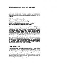
Figure1. Comparison of convergence characteristics of GPSO and PSO-DE.

t

(15)

z i (k )  z i ( k ) t

where zˆ(k ), z (k ) and z t (k ) represent estimated, measured and true values of the measurements , respectively, and m represents the number of measurements used.

4. Results and Discussions The optimized estimators have been tested on all five standard and two ill-conditioned test systems extensively under different normal and bad data measurement conditions. The choice of explicit results to present is difficult as the number of interesting outputs is very large. For the sake of brevity the performance of the proposed SE method has been presented for some of the important results. The results, presented here, can be divided in two distinct categories; one is based on the optimization characteristics of the algorithms and the other is based on the performance characteristics of SE techniques.

4.1. The Optimization Characteristics of Algorithms In Figure 1, the convergence characteristics for IEEE 118-bus test system have been presented for GPSO and PSO-DE based SE. The optimal value of the fitness function of PSO-DE is much less than that of GPSO. In order to check the robustness of the optimization algorithms applied to solve state estimation problem, Copyright © 2013 SciRes.

each technique has been run 100 times and the values of 500th optimization cycle are noted. The results are presented in Table 3. The total range of these values is selected as the difference of maximum values and minimum values. The total range is sub-divided into four equal small sub-ranges viz. Range-1, Range-2, Range-3 and Range-4. The ranges of sub-ranges are shown in Table 3. The comparative study of standard deviations clearly indicates the superiority of the proposed PSO-DE based optimal SE technique. Hence, it can be stated that the PSO-DE based SE has better optimization characteristics of the objective function than the GPSO based SE. Frequency of occurrence (FO) indicates the occurrence of the fitness values in the sub-ranges at the end of 500th optimization cycle. Therefore, the higher FO in the Range-1 indicates the superiority of the algorithm. In Figures 2(a)-(g), the FO values have been plotted against sub-ranges for each test case. From the figure, it is clear that the PSO-DE based SE has higher FO in the Range-1 and lesser FO in other sub-ranges than the same of the GPSO based SE technique. This clearly proves the superiority of the PSO-DE based optimal SE method.

4.2. Performance Characteristics of the SE Techniques In Figure 3, AASE(k) and J(k) indices for 118-bus test system are presented. From the figure, it is clear that the AASE graph of PSO-DE based technique is the closest to EPE

S. MALLICK ET AL.

674

Table 3. Description of ranges of minimum values of objective function and standard deviation of the minimum fitness function values for different test systems for 100 runs of the algorithms. GPSO Test Bus system

Minimum value of objective function

PSO-DE

Maximum Range of value of objective sub-range function values

Standard deviation

Minimum value of objective function

Maximum value of objective function

Range of sub-range values

Standard deviation

IEEE 5-Bus

0.3453

0.5630

0.0551

0.0417

0.0059

0.0350

0.0072

0.0046

IEEE 14-Bus

0.3745

0.8372

0.1541

0.1239

0.0099

0.0282

0.0045

0.0029

IEEE 30-Bus

0.4161

1.5096

0.2733

0.2295

0.0272

0.0414

0.0035

0.0031

IEEE 57-Bus

0.9642

3.1213

0.5392

0.3413

0.0842

0.2881

0.0509

0.0270

IEEE 118-Bus

15.4566

32.1037

4.1617

3.7259

1.8485

3.7460

0.4743

0.3110

11-Bus

5.9385

9.4668

0.8820

0.5958

0.3470

0.8692

0.1305

0.1127

13-Bus

0.1684

0.2427

0.0185

0.0114

0.0024

0.0035

0.0002

0.0002

Figure 2. Comparison of F.O. of the optimal values of objective function for 100th run of the algorithms the GPSO and the PSO-DE based SE. Copyright © 2013 SciRes.

EPE

S. MALLICK ET AL.

675

SE estimates the voltage magnitudes more accurately than the other two techniques. The GPSO based SE predicts the voltage magnitudes slightly better than the standard WLS technique.

5. Conclusions

Figure 3. Comparison of AASE(k) and J(k) obtained by WLS, GPSO and PSO-DE for IEEE 118-Bus test system.

In this paper, hybrid PSO-DE based SE algorithm has been proposed to find the minimum value of fitness function of the SE problem. The proposed method has been tested on IEEE 5-bus, 14-bus, 30-bus, 57-bus and 118-bus standard test systems and 11-bus and 13-bus ill-conditioned test systems extensively for different normal operating conditions and various combinations of bad-data measurement conditions to verify their efficiencies. The results are compared with the same of the standard WLS technique and the GPSO method. From the comparison of results, it has been observed that (i) the PSO-DE based state estimator minimizes the fitness function far better than both GPSO based estimator and WLS based estimator; (ii) the frequency of occurrence of the minimum value near the mean value of the solutions for 100 runs of each algorithm is more in case of the PSO-DE based SE than the GPSO based SE and WLS-SE and (iii) the error analysis study among the three techniques, using AASE(k) and J(k) index, proves the superiority of the PSO-DE based technique over the other two. Comparing all performances, it may thus be concluded that the PSO-DE based state estimation technique shows the best efficiency in state estimation analysis with high accuracy.

REFERENCES Figure 4. Comparative voltage magnitudes of bus number 92 of IEEE 118-Bus test system obtained by WLS, GPSO and PSO-DE.

zero among the three techniques. So, it is obvious that the PSO-DE based technique is more accurate than the GPSO based technique and the WLS-SE technique. WLS has the J(k) values close to 0.8, whereas the GPSO based SE and the PSO-DE based SE provide J(k) values almost constant and parallel to x-axis though the load is varied from 70% to 120%. The effect of inclusion of bad data measurement is overcome in PSO-DE based SE whereas both WLS and the GPSO based estimators cannot eliminate the effect of inclusion of bad data measurement. This clears the superiority of the PSO-DE based SE over the other two techniques. The true values of bus voltage magnitudes obtained using the standard WLS technique, the GPSO based technique and the PSO-DE based technique for load variation of bus number 92 of IEEE 118-bus test system are compared and presented in Figure 4. The PSO-DE based Copyright © 2013 SciRes.

[1]

G. Durgaprasad and S. S. Thakur, “Robust Dynamic State Estimation of Power Systems Based on M-estimation and Realistic Modeling of System Dynamics,” IEEE Transactions Power System, Vol. 13, 1998, pp. 1331-1336. doi:10.1109/59.736273

[2]

F. C. Schweppe and J. Wildes, “Power System Static State Estimation, Part I: Exact Model,” IEEE Transactions Power App. Syst., Vol. PAS-89, 1970, pp. 120-125.

[3]

G. W. Stagg, J. F. Dopazo, A. Klitin and L. S. VanSlyck, “Techniques for the Real-time Monitoring of Power System Operations,” IEEE Transactions Power App. Syst., Vol. PAS-89, No. 4, 1970, pp. 545-555. doi:10.1109/TPAS.1970.292601

[4]

A. Monticelli and F. F. Wu, “Analytical Tools for Power System Restoration-Conceptual design,” IEEE Transactions on Power Apparatus and Systems, Vol. 3, 1988, pp. 201-206.

[5]

A. Monticelli, “Electric Power System State Estimation,” in Proceedings of the, 2000, pp. 1069-1075.

[6]

G. N. Korres, “A Robust Algorithm for Power System State Estimation with Equality Constraints,” IEEE Transactions on Power Apparatus and Systems, Vol. 25,

EPE

S. MALLICK ET AL.

676 No. 3, 2010, pp. 1531-1541. doi:10.1109/TPWRS.2010.2041676 [7]

A. Monticelli and A. Garcia, “Reliable Bad Data Processing for Real-time State Estimation,” IEEE Transactions Power Apparatus and Systems, Vol. PAS-102, 1983, pp. 1126-1139. doi:10.1109/TPAS.1983.318053

[8]

N. G. Bretas, “An Iterative Dynamic State Estimation and Bad Data Processing,” International Journal of Electrical Power and Energy Systems, Vol. 11, 2010, pp. 70-74. doi:10.1016/0142-0615(89)90010-0

[9]

N. G. Bretas, A. S. Bretas and S. A. Piereti, “Innovation Concept for Measurement Gross Error Detection and Identification in Power System State Estimation,” The Institution of Engineering and Technology, Vol. 5, 2011, pp. 603-608. doi:10.1049/iet-gtd.2010.0459

[10] A. M. Sasson, S. T. Ehrmann, P. Lynch, and L. S. Van Slyck, “Automatic Power System Network Topology Determination,” IEEE Transactions Power Apparatus Systems, Vol. PAS-92, No. 2, 1973, pp. 610-618. doi:10.1109/TPAS.1973.293764 [11] K. A. Clements and A. S. Costa, “Topology Error Identification Using Normalized Lagrange Multipliers,” IEEE Transactions Power Systems, Vol. 13, 1998, pp. 347-353. doi:10.1109/59.667350 [12] J. Chen and A. Abur, “Enhanced Topology Error Processing Via Optimal Measurement Design,” IEEE Transactions Power Systems, Vol. 23, 2008, pp. 845-852. doi:10.1109/TPWRS.2008.926083 [13] A. Monticelli and F. F. Wu, “Observability Analysis for Orthogonal Transformation based State Estimation,” IEEE Transactions Power Systems, Vol. PWRS-1, 1986, pp. 201-206. doi:10.1109/TPWRS.1986.4334870 [14] G. N. Korres and P. J. Katsikas, “Reduced Model for Numerical Observability Analysis in Generalised State Estimation,” IET Gener.,Transm. And Distrib., vol. 152, pp. 99-108, 2005. doi:10.1049/ip-gtd:20041059 [15] R. C. Eberhart and J. Kennedy, “A New Optimizer Using Particle Swarm Theory,” in Symposium on Micro Machine and Human Science. Japan: Nagoya, Piscataway, NJ, 1995, pp. 39-43. doi:10.1109/MHS.1995.494215

Copyright © 2013 SciRes.

[16] R. C. Eberhart and Y. Shi, “Comparing Inertia Weights and Constriction Factors in Particle Swarm Optimization,” in Congress on Evolutionary Computation, La Jolla, CA , USA 2000, pp. 84-88. [17] P. Acharjee and S. K. Goswami, “Expert Algorithm Based on Adaptive Particle Swarm Optimization for Power Flow Analysis,” Expert Systems with Applications, Vol. 36, 2009, pp. 5151-5156. doi:10.1016/j.eswa.2008.06.027 [18] Y. Fukuyama and H. Yoshida, “A Particle Swarm Optimization for Reactive Power and Voltage Control in Electrical Power Systems,” in Proc. of 2001 Congress on Evolutionary Computation 2001, pp. 87-93. [19] M. A. Abido, “Optimal Design of Power-system Stabilizers Using Particle Swarm Optimization,” IEEE Transactions on Energy Conversion, Vol. 17, 2002, pp. 406-413. doi:10.1109/TEC.2002.801992 [20] R. Storn and K. Price, "Differential Evolution a Simple and Effective Scheme for Global Optimization over Continuous Spaces,” 1995. [21] T. Hendtlass, “A Combined Swarm Differential Algorithm for Optimization Problems,” in Proceedings of the fourteenth International conference on Industrial and Engineering Applications of Artificial Intelligence and Expert systems, 2001, pp. 11-18. [22] M. G. H. Omran, A. P. Engelbrecht and A. Salman, "Diffeerential evolution based particle swarm optimization," in Proceedings of the IEEE Swarm Intelligence Symposium, 2007, pp. 112-119. [23] B. Shaw, V. Mukherjee and S. P. Ghoshal, “Solution of Combined Economic and Emission Dispatch Problems Using Hybrid Craziness-based PSO with Differential Evolution,” Presented at the IEEE Symposium on Differential Evolution, 2011. [24] S. Mallick, D. V. Rajan, S. S. Thakur, P. Acharjee and S. P. Ghoshal, “Development of a New Algorithm for Power Flow Analysis,” International of Journal of Electtrical Power and Energy Sysems, Vol. 33, 2011, pp. 1479-1488. doi:10.1016/j.ijepes.2011.06.030

EPE