react to relatively simple information higher order invariant features are ..... Localized projections of pure clusters using various projection pursuit indices, ...... These data can be downloaded from the UCI Machine Learning Repository [114]. ...... [44] Baggenstoss, P.: The pdf projection theorem and the class-specific method.
Chapter 1
Optimal Support Features for Meta-learning. Włodzisław Duch1,2 , Tomasz Maszczyk1 , Marek Grochowski1
Abstract Meta-learning has many aspects, but its final goal is to discover in an automatic way many interesting models for a given data. Our early attempts in this area involved heterogeneous learning systems combined with a complexity-guided search for optimal models, performed within the framework of (dis)similarity based methods to discover “knowledge granules”. This approach, inspired by neurocognitive mechanisms of information processing in the brain, is generalized here to learning based on parallel chains of transformations that extract useful information granules and use it as additional features. Various types of transformations that generate hidden features are analyzed and methods to generate them are discussed. They include restricted random projections, optimization of these features using projection pursuit methods, similarity-based and general kernel-based features, conditionally defined features, features derived from partial successes of various learning algorithms, and using the whole learning models as new features. In the enhanced feature space the goal of learning is to create image of the input data that can be directly handled by relatively simple decision processes. The focus is on hierarchical methods for generation of information, starting from new support features that are discovered by different types of data models created on similar tasks and successively building more complex features on the enhanced feature spaces. Resulting algorithms facilitate deep learning, and also enable understanding of structures present in the data by visualization of the results of data transformations and by creating logical, fuzzy and prototype-based rules based on new features. Relations to various machine-learning approaches, comparison of results, and neurocognitive inspirations for meta-learning are discussed. Key words: Machine learning, meta-learning, feature extraction, data understanding Department of Informatics, Nicolaus Copernicus University, Grudzia¸dzka 5, Toru´n, Poland · School of Computer Engineering, Nanyang Technological University, Singapore
1
2
Włodzisław Duch, Tomasz Maszczyk, Marek Grochowski
1.1 Introduction: neurocognitive inspirations for meta-learning Brains are still far better in solving many complex problems requiring signal analysis than computational models. Already in 1855 H. Spencer in the book “Principles of Psychology” discussed associative basis of intelligence, similarity and dissimilarity, relations between physical events, “psychical changes”, and activity of brain parts (early history of connectionism is described in [1]). Why are brains so good in complex signal processing tasks, while machine learning is so poor, despite development of sophisticated statistical, neural network and other biologically-inspired computational intelligence (CI) algorithms? Artificial neural networks (ANNs) drew inspiration from neural information processing at single neuron level, initially treating neurons as threshold logic devices, later adding graded response (sigmoidal) neurons [2] and finally creating detailed spiking neural models that are of interest mainly to people in computational neuroscience [3]. Attempts to understand microcircuits and draw inspirations from functions of whole neocortical columns have so far not been too successful. The Blue Brain Project [4] created biologically accurate simulation of neocortical columns, but the project did not provide any general principles how these columns operate. Computational neuroscience is very important to understand details of neural functions, but may not be the shortest way to computational intelligence. Situation in computational quantum physics and chemistry is analogous: despite detailed simulations of molecular properties little knowledge useful for conceptual thinking has been generated. Neurocognitive inspirations for CI algorithms based on general understanding of brain functions may be quite useful. Intelligent systems should have goals, select appropriate data, extract information from data, create percepts and reason using information derived from them. Goal setting may be a hierarchical process, with many subgoals forming a plan of action or solution to a problem. Humans are very flexible in finding alternative solutions, but current CI methods are focused on searching for a single best solutions. Brains search for alternative solutions recruiting many specialized modules, some of which are used only in very unusual situations. A single neocortical column provides many types of microcircuits that respond in a qualitatively different way to the incoming signals [5]. Other cortical columns may combine these responses in a hierarchical way creating complex hidden features based on information granules extracted from all tasks that may benefit from such information. General principles, such as complementarity of information processed by parallel interacting streams with hierarchical organization are quite useful [6]. Neuropsychological models of decision making assume that noisy stimulus information from multiple parallel streams is accumulated until sufficient information is obtained to make reliable response [7]. Decisions may be made if sufficient number of features extracted by information filters provide reliable information. Neurocognitive principles provide an interesting perspective on recent activity in machine learning and computational intelligence. In essence, learning may be viewed as a composition of transformations, with parallel streams that discover basic features in the data, and recursively combine them in new parallel streams of
1 Optimal Support Features for Meta-learning.
3
higher-order features, including high-level features derived from similarity to memorized prototypes or categories at some abstract level. In the space of such features knowledge is transferred between different tasks and used in solving problems that require sequential reasoning. Neurocognitive inspirations provide a new perspective on: Liquid State Machines [5], ”reservoir computing” [8], deep learning architectures [9], deep belief networks [10], kernel methods [11], boosting methods that use week classifiers [12], ensemble learning [13, 14], various meta-learning approaches [15], regularization procedures in feedforward neural networks, and many other machine learning areas. The key to understanding general intelligence may lie in specific information filters that make learning possible. Such filters have been developed slowly by the evolutionary processes. Integrative chunking processes [16] combine this information into higher-level mental representations. Filters based on microcircuits discover phonemes, syllables, words in the auditory stream (with even more complex hierarchy in the visual stream), lines and edges, while chunking links sequences of lower level patterns into single higher-level patterns, discovering associations, motifs and elementary objects. Meta-learning tries to reach this level of general intelligence providing additional level of control to search for composition of various transformations, including whole specialized learning modules, that “break and conquer” difficult tasks into manageable subproblems. The great advantage of Lisp programming is that the program may modify itself. There are no examples of CI programs that could adjust themselves in a deeper way, beyond parameter optimization, to the problem analyzed. Constructive algorithms that add new transformations as nodes in a graphic model are a step in this direction. Computational intelligence tries to create universal learning systems, but biological organisms frequently show patterns of innate behavior that are useful only in rare, quite specific situations. Models that are not working well on all data, but work fine in some specific cases should still be useful. There is “no free lunch” [17], no single system may reach the best results for all possible distributions of data. Therefore instead of a direct attempt to solve all problems with one algorithm, a good strategy is to transform them into one of many formulations that can be handled by selected decision models. This is possible only if relevant information that depends on the set goal is extracted from the input data stream and is made available for decision processes. If the goal is to understand data (making comprehensible model of data), algorithms that extract interesting features from raw data and combine them into rules, find interesting prototypes in the data or provide interesting visualizations of data should be preferred. A lot of knowledge about reliability of data samples, possible outliers, suspected cases, relative costs of features or their redundancies is usually ignored as there is no simple way to use it in the CI programs. Such information is needed to set the meta-learning goals. Many meta-learning techniques have recently been developed to deal with the problem of model selection [15, 18]. Most of them search for optimal model characterizing a given problem by some meta-features (e.g. statistical properties, landmarking, model-based characterization), and by referring to some meta-knowledge gained earlier. For a given data one can use the classifier that gave the best result on
4
Włodzisław Duch, Tomasz Maszczyk, Marek Grochowski
a similar dataset in the StatLog Project [19]. However, choosing good meta-features is not a trivial issue as most features do not characterize the complexity of data distributions. In addition the space of possible solutions generated by this approach is bounded to already known types of algorithms. The challenge is to create flexible systems that can extract relevant information and reconfigure themselves finding many interesting solutions for a given task. Instead of a single learning algorithm designed to solve specialized problem, priorities are set to define what makes an interesting solution, and a search for configurations of computational modules that automatically create algorithms on demand should be performed. This search in the space of all possible models should be constrained by user priorities and should be guided by experience with solving problems of similar nature, experience that defines “patterns of algorithm behavior” in problem solving. Understanding visual or auditory scenes is based on experience and does not seem to require much creativity, even simple animals are better at it than artificial systems. With no prior knowledge about a given problem finding an optimal sequence of transformations may not be possible. Meta-learning based on these ideas requires several components: • specific filters extracting relevant information from raw data, creating useful support features; • various compositions of transformations that create higher-order features analyzing patterns in enhanced feature spaces; • models of decision processes based on these high-order features; • intelligent organization of search that discovers new models of decision processes, learning from previous attempts. At the meta-level it may not be important that a specific combination of features proved to be successful in some task, but it is important that a specific transformation of a subset of features was once useful, or that distribution of patterns in the feature space had some characteristics that may be described by some specific data model and is easy to adapt to new data. Such information allows for generalization of knowledge at the level of search patterns for a new composition of transformations, facilitating transfer of knowledge between different tasks. Not much is known about the use of heuristic knowledge to guide the search for interesting models and our initial attempts to meta-learning, based on the similarity framework [20, 21] used only simple greedy search techniques. The Metal project [22] tried to collect information about general data characteristics and correlate it with the methods that performed well on a similar data. A system recommending classification methods has been built using this principle, but it works well only in a rather simple cases. This paper is focused on generation of new features that provide good foundation for meta-learning, creating information on which search processes composing appropriate transformations may operate. The raw features given in the dataset description are used to create a large set of enhanced or hidden features. The topic of feature generation has received recently more attention in analysis of sequences and images, where graphical models known as Conditional Random Fields became popular [23], generating for natural text analysis sometimes millions of low-level
1 Optimal Support Features for Meta-learning.
5
features [24]. Attempts at meta-learning on the ensemble level lead to very rough granularity of the existing models and knowledge [25], thus exploring only a small subspace of all possible models, as it is done in the multistrategy learning [26]. Focusing on generation of new features leads to models that have fine granularity of the basic building blocks and thus are more flexible. We have partially addressed this problem in the work on heterogeneous systems [27–34]. Here various types of potentially useful features are analyzed, including higher-order features. Visualization of the image of input data in the enhanced feature space helps to set the priority for application of models that worked well in the past, learning how to transfer metaknowledge about the types of transformations that have been useful, and transferring this knowledge to new cases. In the next section various transformations that extract information forming new features are analyzed. Section three shows how transformation based learning may benefit from enhanced feature spaces, how to define goals of learning and how to transfer knowledge between learning tasks. Section four shows a few lessons from applying this line of thinking to real data. The final section contains discussion and conclusions.
1.2 Extracting Features for Meta-Learning Brains do not attempt to recognize all objects in the same feature space. Even within the same sensory modality a small subset of complex features is selected, allowing to distinguish one class of objects from another. While the initial receptive fields react to relatively simple information higher order invariant features are extracted from signals as a result of hierarchical processing of multiple streams of information. Object recognition or category assignment by the brain is probably based on evaluation of similarity to memorized prototypes of objects using a few characteristic features [35], but for different classes of objects these features may be of quite different type, i.e. they are class specific. Using different complex features in different regions of the input space may drastically simplify categorization problems. This is possible in hierarchical learning models, graphical models, or using conditionally defined features (see section 1.2.8). Almost all adaptive learning systems are homogeneous, based on elements extracting information of the same type. Multilayer Perceptron (MLP) neural networks use nodes that partition the input space by hyperplanes. Radial Basis Function networks based on localized functions frequently use nodes that provide spherical or ellipsoidal decision borders [36]. Similarity-based methods use the same distance function for each reference vector, decision trees use simple tests based on thresholds or subsets of values creating hyperplanes. Support Vector Machines use kernels globally optimized for a given dataset [37]. This cannot be the best inductive bias for all data, frequently requiring large number of processing elements even in cases when simple solutions exist. The problem has been addressed by development of various heterogenous algorithms [31] for neural networks [27–29],neurofuzzy sys-
6
Włodzisław Duch, Tomasz Maszczyk, Marek Grochowski
tems [30], decision trees [32] and similarity-based systems [33, 34, 38, 39] and multiple kernel learning methods [40]. Class-specific high order features emerge naturally in hierarchical systems, such as decision trees or rule-based systems [41, 42], where different rules or branches of the tree use different features (see [43, 44]). The focus of neural network community has traditionally been on learning algorithms and network architectures, but it is clear that selection of neural transfer functions determines the speed of convergence in approximation and classification problems [27, 45, 46]. The Pfamous n-bit parity problem is trivially solved using a periodic function cos(ω i bi ) with a single parameter ω and projection of the bit strings on weight vector with identical values W = [1, 1, ..1], while the multilayer perceptron (MLP) networks need O(n2 ) parameters and have great difficulty to learn such functions [47]. Neural networks are non-parametric universal approximators but the ability to learn requires flexible “brain modules”, or transfer functions that are appropriately biased for the problem being solved. Universal learning methods should be non-parametric but they may be heterogeneous. Initial feature space for a set of objects O is defined by direct observations, measurements, or estimations of similarity to other objects, creating the vector of raw input data 0 X(O) = X(O). These vectors may have different length and in general some structure descriptors, grouping features of the same type. Learning from such data is done by a series of transformations that generate new, higher order features. Several types of transformations of input vectors should be considered: component, selector, linear combinations and non-linear functions. Component transformations, frequently used in fuzzy modeling [48], work on each input feature separately, scaling, shifting, thresholding, or windowing raw features. Each raw feature may give rise to several new features suitable for calculations of distances, scalar products, membership functions and non-linear combinations at the next stage. Selector transformations define subsets of vectors or subsets of features using various criteria for information selection, distribution of feature values and class labels, or similarity to the known cases (nearest neighbors). Non-linear functions may serve as kernels or as neural transfer functions [27]. These elementary transformations are conveniently presented in a network form. Initial transformations T1 of raw data should enhance information related to the learning goals carried by new features. At this stage combining small subsets of features using Hebbian learning based on correlations is frequently most useful. A new dataset 1 X = T1 (0 X) forms an image of the original data in the space spanned by a new set of features. Depending on the data and goals of learning, this space may have dimensionality that is smaller or larger than the original data. The second transformation 2 X = T2 (1 X) usually extracts multidimensional information from pre-processed features 1 X. This requires an estimation which of the possible transformations at the T1 level may extract information that will be useful for specific T2 transformations. Many aspects can be taken into account defining such transformations, as some types of features are not appropriate for some learning models and optimization procedures. For example, binary features may not work well with gradient based optimization techniques, and standardization may not help if rule-based solutions are desired. Intelligent search procedures in meta-learning schemes should
1 Optimal Support Features for Meta-learning.
7
take such facts into account. Subsequent transformations may use T2 as well as T1 and the raw features. The process is repeated until the final transformation is made, aimed either at separation of the data, or at mapping to a specific structures that can be easily recognized by available decision algorithms. Higher-order features created after a series of k transformations k Xi should also be treated in the same way as raw features. All features influence the geometry of decision regions; this perspective helps to understand their advantages and limitations. All these transformations can be presented in a graphical form. Meta-learning needs also to consider computational costs of different transformations.
1.2.1 Extracting Information from Single Features Preprocessing may critically influence convergence of learning algorithms and construction of the final data models. This is especially true in meta-learning, as the performance of various methods if facilitated by different transformations, and it may be worthwhile to apply many transformations to extract relevant information from each feature. Raw input features may contain useful information, but not all algorithms include preprocessing filters to access it easily. How are features 1 Xij = T1j (0 Xi ), created from raw features 0 Xi applying transformation T1j , used by the next level of transformations? They are either used in an additive way in linear combinations for weighted products, or in distance/similarity calculation, or in multiplicative way in probability estimation, or as a logical condition in rules or decision trees with suitable threshold for its value. Methods that compute distances or scalar products benefit from normalization or standardization of feature values. Using logarithmic, sigmoidal, exponential, polynomial and other simple functions to make density of points in one dimension more uniform may sometimes help to circumvent problems that require multiresolution algorithms. Standardization is relevant to additive use of features in distance calculation (nearest neighbor methods, most kernel methods, RBF networks), it also helps to initialize weights in linear combinations (linear discrimination, MLP), but is not needed for logical rules/decision trees. Fuzzy and neurofuzzy systems usually include a “fuzzification step”, defining for each feature several localized membership functions µk (Xi ) that act as receptive fields, filtering out the response outside the range of significant values of the membership functions. These functions are frequently set in an arbitrary way, covering the whole range of feature values with several membership functions that have triangular, Gaussian or similar shapes. This is not the best way to extract information from single features [41]. Filters that work as receptive fields separate subsets or ranges of values that should be correlated with class distribution [49], “perceiving” subsets or intervals where one of the classes dominate. If the correlation of feature values in some interval [Xia , Xib ], or a subset of values with some target output is strong membership function µab (Xi ) covering these values is useful. This implies that it is not necessary to replace all input features by their fuzzified versions. Class-
8
Włodzisław Duch, Tomasz Maszczyk, Marek Grochowski
conditional probabilities P(C|Xi ), as computed by Naive Bayes algorithms, may be used to identify ranges of Xi feature values where a single class dominates, providing optimal membership functions µk (Xi ) = P(C|Xi )/P(Xi ). Negative information, i.e. information about the absence of some classes in certain range of feature values, should also be segmented: if P(Ck |Xi ) < � in some interval [Xia , Xib ] then a derived feature Hikab (Xi ), where H(·) is a window-type function, carries valuable information that higher order transformations are able to use. Eliminators may sometimes be more useful than classifiers [50]. Projecting each feature value Xi on these receptive fields µk increases the dimensionality of the original data, increasing a chance of finding simple models of the data in the enhanced space.
1.2.2 Binary Features Binary features Bi are the simplest, indicating presence or absence of some observations. They may also be created dividing nominal features into two subsets, or creating subintervals of real features {Xi }. Using filter methods [49], or such algorithms as 1R [51] or Quality of Projected Clusters [52], intervals of real feature values that are correlated with the targets may be selected and presented as binary features. From geometrical perspective binary feature is a label distinguishing two subspaces, projecting all vectors in each subspace on a point 0 or 1 on the coordinate line. The vector of n such features corresponds to all 2n vertices of the hypercube. Feature values are usually defined globally, for all available data. Some features are useful only locally in specific context. From geometrical perspective they are projections of vectors that belong to subspaces where specific conditions are met, and should remain undefined for all other vectors. Such conditionally defined features frequently result from questionnaires: if the answer to the last question was yes, then give additional information. In this case for each value Bi = 0 and Bi = 1 subspaces have different dimensionality. The presence of such features is incorporated in a natural way in graphical models [53], such as Conditional Random Fields [23], but the inference process is then more difficult than using the flat data where standard classification techniques are used. Enhancing the feature space by adding conditionally defined features may not be so elegant as using the full power of graphical techniques but can go a long way towards improving the results. Conditionally defined binary features may be obtained by imposing various restrictions on vector subspaces used for projections. Instead of using directly the raw feature Bi conditions Bi = T ∧ LTi (X), and Bi = F ∧ LFi (X) are added, where LT (X), LF (X) are logical functions defining the restrictions using feature vector X. For example, other binary features may create complexes LT = B2 ∧ B3 ... ∧ Bk that help to distinguish interesting regions more precisely. Such conditional binary features are created by branch segments in a typical decision tree, for example if one of the path at the two top levels is X1 < t1 ∧ X2 ≥ t2 , then this defines a subspace containing all vectors for which this condition is true, and in which the third and higher level features are defined.
1 Optimal Support Features for Meta-learning.
9
Such features have not been considered in most learning models, but for problems with inherent logical structure decision trees and logical rules have appropriate bias [41, 42] and thus are a good source for generation of conditionally defined binary features. Similar considerations may be done for nominal features that may sometimes be grouped into larger subsets, and for each value restrictions on their projections applied.
1.2.3 Real-valued Features From geometrical perspective the real-valued input features acquired from various tests and measurements on a set of objects are a projection of some property on a single line. Enhancement of local contrast is very important in natural perception. Some properties directly relevant to the learning task may increase their usefulness after transformation by a non-linear sigmoidal function σ(βXi − ti ). Slopes β and thresholds ti may be individually optimized using mutual information or other relevance measures independently for each feature. Single features may show interesting patterns of p(C|X) distributions, for example a periodic distribution, or k pure clusters. Projections on a line that show k-separable data distributions are very useful for learning complex Boolean functions. For n-bit parity problem n + 1 separate clusters may be distinguished in projections on the long diagonal, forming useful new features. A single large cluster of pure values is worth turning into a new feature. Such features are generated by applying bicentral functions (localized window-type functions) to original features [52], for example Zi = σ(Xi − ai ) − σ(Xi − bi ), where ai > bi . Changing σ into a step function will lead to a binary features, filtering vectors for which logical condition Xi ∈ [ai , bi ] is true. Soft σ creates window-like membership functions, but may also be used to create higher-dimensional features, for example Z12 = σ(t1 − X1 )σ(X2 − t2 ). Providing diverse receptive fields for sampling the data separately in each dimension is of course not always sufficient, as two or higher-dimensional receptive fields are necessary in some applications, for example in image or signal processing filters, such as wavelets. Q For real-valued features simplest constraints are made by products of intervals i [ri− , ri+ ], or product of bicentral functions defining hyperboxes in which projected vectors should lie. Other ways to restrict subspaces used for projection may be considered, for example taking only vectors that are in a cylindrical area surrounding the X1 coordinate Z1d = σ(X1 − t1 )σ(d − ||X||−1 ), where ||X||−1 norm excludes X1 feature. The point here is that transformed features should label different regions of feature space simplifying the analysis of data in these regions.
10
Włodzisław Duch, Tomasz Maszczyk, Marek Grochowski
1.2.4 Linear Projections Groups of several correlated features may be replaced by a single combination performing principal component analysis (PCA) restricted to small subspaces. To decide which groups should be combined standardized Pearson’s linear correlation is calculated: |Cij | ∈ [−1, +1] (1.1) rij = 1 − σi σj where the covariance matrix is: n �� � 1 X � (k) ¯ i X (k) − X ¯j ; Xi − X Cij = j n−1
i, j = 1 · · · d
(1.2)
k=1
Correlation coefficients may be clustered using dendrogram or other techniques. Linear combinations of strongly correlated features allow not only for dimensionality reduction, but also for creation of features at different scales, from a combination of a few features, to a global PCA combinations of all features. This approach may help to discover hierarchical sets of features that are useful in problems requiring multiscale analysis. Another way to obtain features for multiscale problems is to do clusterization in the input data space and make local PCA within the clusters to find features that are most useful locally in various areas of space. Exploratory Projection Pursuit Networks (EPPNs) [54, 55] is a general technique that may be used to define transformations creating new features. Quadratic cost functions used for optimization of linear transformations may lead to formulation of the problem in terms of linear equations, but most cost functions or optimization criteria are non-linear even for linear transformations. A few unsupervised transformations are listed below: • Principal Component Analysis (PCA) in its many variants provides features that correspond to feature space directions with the highest variance [17, 56, 57]. • Independent Component Analysis provides features that are statistically independent [58, 59]. • Classical scaling, or linear transformation embedding input vectors in a space where distances are preserved [60]. • Factor analysis, computing common and unique factors. Many supervised transformations may be used to determine coefficients for combination of input features, as listed below. • Any measure of dependency between class and feature value distributions, such as the Pearson’s correlation coefficient, χ2 , separability criterion [61], • Information-based measures [49], such as the mutual information between classes and new features [62], Symmetric Uncertainty Coefficient, or KullbackLeibler divergence.
1 Optimal Support Features for Meta-learning.
11
• Linear Discriminatory Analysis (LDA), with each feature based on orthogonal LDA direction obtained by one of the numerous LDA algorithms [17, 56, 57], including linear SVM algorithms. • Fisher Discriminatory Analysis (FDA), with each node computing canonical component using one of many FDA algorithms [56, 63]. • Linear factor analysis, computing common and unique factors from data [64]. • Canonical correlation analysis [65]. • Localized projections of pure clusters using various projection pursuit indices, such as the Quality of Projected Clusters [52]. • General projection pursuit transformations [54, 55] provide a framework for various criteria used in searching for interesting transformations. Many other transformations of this sort are known and may be used at this stage in transformation-based systems. The Quality of Projected Clusters (QPC) is a projection pursuit method that is based on a leave-one-out estimator measuring quality of clusters projected on W direction. The supervised version of this index is defined as [52]: QP C(W) = (1.3) X X X � � A+ G WT (X − Xk ) − A− G WT (X − Xk ) X
Xk ∈CX
Xk ∈C / X
where G(x) is a function with localized support and maximum for x = 0 (e.g. a Gaussian function), and CX denotes the set of all vectors that have the same label as X. Parameters A+ , A− control influence of each term in Eq. (1.3). For large value of A− strong separation between classes is enforced, while increasing A+ impacts mostly compactness and purity of clusters. Unsupervised version of this index may simply try to discover projection directions that lead to separated clusters. This index achieves maximum value for projections on the direction W that group vectors belonging to the same class into a compact and well separated clusters. Therefore it is suitable for multi-modal data [47]). The shape and width of the G(x) function used in E.q. (1.3) has influence on convergence. For continuous functions G(x) gradient-based methods may be used to maximize the QPC index. One good choice is an inverse quartic function: G(x) = 1/(1 + (bx)4 ), but any bell-shaped function is suitable here. Direct calculation of the QPC index (1.3), as in the case of all nearest neighbor methods, requires O(n2 ) operations, but fast version, using centers of clusters instead of pairs of vectors, has only O(n) complexity (Grochowski and Duch, in print). The QPC may be used also (in the same way as the SVM approach described above) as a base for creation of feature ranking and feature selection methods. Projection coefficients Wi indicate then significance of the i-th feature. For noisy and non-informative variables values of associated weights should decrease to zero during QPC optimization. Local extrema of the QPC index may provide useful insight into data structures and may be used in a committee-based approach that combines different views on the
12
Włodzisław Duch, Tomasz Maszczyk, Marek Grochowski
same data. More projections are obtained repeating procedure in the orthogonalized space to create sequence of unique interesting projections [52]. Srivastava and Liu [66] analyzed optimal transformations for different applications presenting elegant geometrical formulation using Stiefel and Grassmann manifolds. This leads to a family of algorithms that generate orthogonal linear transformations of features, optimal for specific tasks and specific datasets. PCA seems to be optimal transformation for image reconstruction under mean-squared error, Fisher discriminant for classification using linear discrimination, ICA for signal extraction from a mixture using independence, optimal linear transformation of distances for the nearest neighbor rule in appearance-based recognition of objects, transformations for optimal generalization (maximization of margin), sparse representations of natural images and retrieval of images from a large database. In all these applications optimal transformations are different and may be found by optimizing appropriate cost functions. Some of the cost functions advocated in [66] may be difficult to optimize and it is not yet clear that sophisticated techniques based on differential geometry offer significant practical advantages. Simpler learning algorithms based on numerical gradient techniques and systematic search algorithms give surprisingly good results and can be applied to optimization of difficult functions [67].
1.2.5 Kernel Features The most popular type of SVM algorithm with localized (usually Gaussian) kernels [11] suffers from the curse of dimensionality [68]. This is due to the fact that such algorithms rely on assumption of uniform resolution and local similarity between data samples. To obtain accurate solution often a large number of training examples used as support vectors is required. This leads to high cost of computations and complex models that do not generalize well. Much effort has been devoted to improvements of the scaling [69, 70], reducing the number of support vectors, [71], and learning multiple kernels [40]. All these developments are impressive, but there is still room for simpler, more direct and comprehensible approaches. In general the higher the dimensionality of the transformed space the greater the chance that the data may be separated by a hyperplane [36]. One popular way of creating highly-dimensional representations without increasing computational costs is by using the kernel trick [11]. Although this problem is usually presented in the dual space the solution in the primal space is conceptually simpler [70, 72]. Regularized linear discriminant (LDA) solution is found in the new feature space 2 X = K(X) = K(1 X, X), mapping X using kernel functions for each training vector. Kernel methods work because they implicitly provide new, useful features Zi (X) = K(X, Xi ) constructed by taking the support vectors Xi as reference. Linear SVM solutions in the Z kernel feature space are equivalent to the SVM solutions, as it has been empirically verified [73]. Feature selection techniques may be used to leave only components corresponding to “support vectors” that provide essential support for classification, for example
1 Optimal Support Features for Meta-learning.
13
only those that are close to the decision borders or those close to the centers of cluster, depending on the type of the problem. Once a new feature is proposed it may be evaluated on vectors that are classified at a given stage with low confidence, thus ensuring that features that are added indeed help to improve the system. Any CI method may be used in the kernel-based feature space K(X). This is the idea behind Support Feature Machines [73]. If the dimensionality is large data overfitting is a big danger, therefore only the simplest and most robust models should be used. SVM solution to use LDA with margin maximization is certainly a good strategy. Explicit generation of features based on different similarity measures [39] removes one of the SVM bottleneck allowing for optimization of resolution in different areas of the feature space, providing strong non-linearities where they are needed (small dispersions in Gaussian functions), and using smooth functions when this is sufficient. This technique may be called adaptive regularization, in contrast to a simple regularization based on minimization of the norm of the weight vector ||W|| used in SVM or neural networks. Although simple regularization enforces smooth decision borders decreasing model complexity it is not able to find the simplest solutions and may easily miss the fact that a single binary feature contains all information. Generation of kernel features should therefore proceed from most general, placed far from decision border (such vectors may be easily identified by looking at the z = W · X distribution for W = (m1 − m2 )/||m1 − m2 ||, where m1 and m2 denote center points of two opposite classes), to more specific, with non-zero contribution only close to decision border. If dispersions are small many vectors far from decision borders have to be used to create kernel space, otherwise all such vectors, independently of the class, would be mapped to zero point (origin of the coordinate system). Adding features based on linear projections will remove the need for support vectors that are far from decision borders. Kernel features based on radial functions are projections on one radial dimension and in this sense are similar to the linear projections. However, linear projections are global and position independent, while radial projections use reference vector K(X, R) = ||X − R|| that allows for focusing on the region close to R. Additional scaling factors are needed to take account of importance of different features K(X, R; W) = ||W · (X − R)||. If Gaussian kernels are used this leads to features of the G(W(X − R)) type. More sophisticated features are based on Mahalanobis distance calculated for clusters of vectors located near decision borders (an inexpensive method for rotation of density functions with d parameters has been introduced in [27]), or flat local fronts using cosine distance. There is a whole range of features based on projections on more than one dimension. Mixed “cylindrical” kernel features that are partially radial and partially linear may also be considered. Assuming that ||W || = 1 linear projection y = W · X defines one direction in the n-dimensional feature space, and at each point y projections are made from the remaining n − 1 dimensional subspaces orthogonal to W, such that ||X − yW|| < θ, forming a cylinder in the feature space. In general projections may be confined to k-dimensional hyperplane and radial dimensions to the (n − k)-dimensional subspace. Such features have never been systematically analyzed and there are no algorithms aimed at their extraction. They are conditionally
14
Włodzisław Duch, Tomasz Maszczyk, Marek Grochowski
defined in a subspace of the whole feature space, so for some vectors they are not relevant.
1.2.6 Other Non-Linear Mappings Linear combinations derived from interesting projection directions may provide low number of interesting features, but in some applications non-linear processing is essential. The number of possible transformations in such case is very large. Tensor products of features are particularly useful, as Pao has already noted introducing functional link networks [74, 75]. Rational function neural networks [36] in signal processing [76] and other applications use ratios of polynomial combinations of features; a linear dependence on a ratio y = x1 /x2 is not easy to approximate if the two features x1 , x2 are used directly. The challenge is to provide a single framework for systematic selection and creation of interesting transformations in a meta-learning scheme. Linear transformations in the kernel space are equivalent to non-linear transformations in the original feature space. A few non-linear transformations are listed below: • Kernel versions of linear transformations, including radial and other basis set expansion methods [11]. • Weighted distance-based transformations, a special case of general kernel transformations, that use (optimized) reference vectors [39]. • Perceptron nodes based on sigmoidal functions with scalar product or distancebased activations [77, 78], as in layers of MLP networks, but with targets specified by some criterion (any criterion used for linear transformations is sufficient). • Heterogeneous transformations using several types of kernels to capture details at different resolution [27]. • Heterogeneous nodes based or several type of non-linear functions to achieve multiresolution transformations [27]. • Nodes implementing fuzzy separable functions, or other fuzzy functions [79]. • Multidimensional scaling (MDS) to reduce dimensionality while preserving distances [80]. MDS requires costly minimization to map new vectors into reduced space; linear approximations to multidimensional scaling may be used to provide interesting features [60]. If highly nonlinear low-dimensional decision borders are needed large number of neurons should be used in the hidden layer, providing linear projection into high-dimensional space followed by squashing by the neural transfer functions to normalize the output from this transformation.
1 Optimal Support Features for Meta-learning.
15
1.2.7 Adaptive Models as Features Meta-learning usually leads to several interesting models, as different types of features and optimization procedures used by the search procedure may create roughly equivalent description of individual models. The output of each model may be treated as a high-order feature. This reasoning is motivated both from the neurocognitive perspective, and from the machine learning perspective. Attention mechanisms are used to save energy and inhibit parts of the neocortex that are not competent in analysis of a given type of signal. All sensory inputs (except olfactory) travel through the thalamus where their importance and rough category is estimated. Thalamic nuclei activate only those brain areas that may contribute useful information to the analysis of a given type of signals [81]. Usually new learning methods are developed with the hope that they will be universally useful. However, evolution has implanted in brains of animals many specialized behaviors, called instincts. From the machine learning perspective a committee of models should use diverse individual models specializing in analysis of different regions of the input space, especially for learning difficult tasks. Individual models are frequently unstable [82], i.e. quite different models are created as a result of repeated training (if learning algorithms contains stochastic elements) or if the training set is slightly perturbed [83]. The mixture of models allows for approximation of complicated probability distributions improving stability of individual models. Specialized models that handle cases for which other models fail should be maintained. In contrast to boosting [12] and similar procedures [84] explicit information about competence of each model in different regions of the feature space should be used. Functions describing these regions of competence (or incompetence) may be used for regional boosting [85] or for integration of decisions of individual models [14, 86]. The same may be done with some features that are useful only in localized regions of space but should not be used in other regions. In all areas where some feature or the whole model Ml works well the competence factor should reach F (X; Ml ) ≈ 1 and it should decrease to zero in regions where many errors are made. A Gaussian-like function may be used, F (||X − Ri ||; Ml ) = 1 − G(||X − Ri ||a ; σi ), where a ≥ 1 coefficient is used to flatten the function, or a simpler 1/ (1 + ||X − Ri ||−a ) inverse function, or a logistic function 1 − σ(a(||X − Ri || − b)), where a defines its steepness and b the radius where the value drops to 1/2. Multiplying many factors in the incompetence function of the model may decrease the competence values, therefore each factor should quickly reach 1 outside the incompetence area. This is achieved by using steep functions or defining a threshold values above which exactly 1 is taken. The final decision based on results of all l = 1 . . . m models providing estimation of probabilities P(Ci |X; Ml ) for i = 1 . . . K classes may be done using majority voting, averaging results of all models, selecting a single model that shows highest confidence (i.e. gives the largest probability), selecting a subset of models with confidence above some threshold, or using simple linear combination [13]. In
16
Włodzisław Duch, Tomasz Maszczyk, Marek Grochowski
the last case for class Ci coefficients of linear combination are determined from the least-mean square solution of:
P(Ci |X; M ) = =
m X X l=1 m m X X
Wi,l (X)P(Ci |X; Ml )
(1.4)
Wi,l F (X; Ml )P(Ci |X; Ml )
l=1 m
The incompetence factors simply modify probabilities F (X; Ml )P(Ci |X; Ml ) that are used to set linear equations for all training vectors X, therefore the solution is done in the same way as before. The P final probability of classification is estimated by renormalization P(Ci |X; M )/ j P(Cj |X; M ). In this case results of each model are used as high order feature for local linear combination of results. This approach may also be justified using neurocognitive inspirations: thalamocortical loops control which brain areas should be strongly activated depending on their predicted competence. In different regions of the input space (around reference vector R) kernel features K(X, R) that use weighted distance functions should have zero weights for those input features that are locally irrelevant. Many variants of committee or boosting algorithms with competence are possible [13], focusing on generation of diversified models, Bayesian framework for dynamic selection of most competent classifier [87], regional boosting [85], confidence-rated boosting predictions [12], task clustering and gating approach [88], or stacked generalization [89, 90].
1.2.8 Summary of the Feature Types Features are weighted and combined by distance functions, kernels, hidden layers, and in many other ways, but geometrical perspective shows what kind of information can be extracted from them. What types of subspaces and hypersurfaces that contained them are generated? An attempt to categorize different types of features from this perspective, including conditionally defined features, is shown below. X represents here arbitrary type of scalar feature, B is binary, N nominal, R continuous real valued, K is general kernel feature, M are motifs in sequences, and S are signals. • B1) Binary, equivalent to unrestricted projections on two points. • B2) Binary, constrained by other binary features, complexes B1 ∧ B2 ... ∧ Bk , subsets of vertices of a cube. • B3) Binary, projection of subspaces constrained by a distance B = 0 ∧ R1 ∈ [r1− , r1+ ]... ∧ Rk ∈ [rk− , rk+ ]. • N1-N3) Nominal features are similar to binary with subsets instead of intervals.
1 Optimal Support Features for Meta-learning.
17
• R1) Real, equivalent to unrestricted orthogonal projections on a line, with thresholds and rescaling. • R2) Real, orthogonal projections on a line restricted by intervals or soft membership functions, selecting subspaces orthogonal to the line. • R3) Real, orthogonal projections with cylindrical constrains restricting distance from the line. • R4) Real, any optimized projection pursuit on a line (PCA, ICA, LDA, QPC). • R5) Real, any projection on a line with periodic or semi-periodic intervals or general 1D patterns, or posterior probabilities for each class calculated along this line p(C|X). • K1) Kernel features K(X, Ri ) with reference vectors Ri , projections on a radial coordinate creating hyperspheres. • K2) Kernel features with intervals, membership functions and general patterns on a radial coordinate. • K3) General kernel features for similarity estimation of structured objects. • M1) Motifs, based on correlations between elements and on sequences of discrete symbols. • S1) Signal decompositions and projections on basis functions. • T1) Other non-linear transformations restricting subspaces in a more complex way, rational functions, universal transfer functions. Combinations of different types of features, for example cylindrical constraints with intervals or semi-periodic functions are also possible. The classification given above is not very precise and far from complete, but should give an idea what type of decision borders may be generated by different types of features. Higher-order features may be build by learning machines using features that have been constructed by earlier transformations. Relevance indices applied to these features, or feature selection methods, should help to estimate their importance, although some features may be needed for local representation of information only, so their global relevance may be low [49].
1.3 Transformation-based meta-learning A necessary step for meta-learning is to create taxonomy, categorizing and describing similarities and relations among transformations and facilitate systematic search in the space of all possible compositions of these transformations. An obvious division is between transformations optimized locally with well-defined targets, and adaptive transformations that are based on a distal criteria, where the targets are defined globally, for composition of transformations (as in backpropagation). In the second case interpretation of features implemented by hidden nodes is rather difficult. In the first case activity of the network nodes implementing fixed transformations has clear interpretation, and increased complexity of adding new node should be justified by discovery of new aspects of the data. Local T2 transformations have
18
Włodzisław Duch, Tomasz Maszczyk, Marek Grochowski
coefficients calculated directly from the input data or data after T1 transformation. They may be very useful for initialization of global adaptive transformations, or may be useful to find better solutions of more complex fixed transformations. For example, multidimensional scaling requires very difficult minimization and most of the time converges to a better solution if PCA transformations is performed first. After initial transformations all data is converted to internal representation k X, forming a new image of the data, distributed in a simpler way than the original image. The final transformation should be able to extract desired information form this image. If the final transformation is linear Y = k+1 X = Tk+1 (k X; k W) parameters k W are either determined in an iterative procedure simultaneously with all other parameters W from previous transformations (as in the backpropagation algorithms [36]), or sequentially determined by calculating the pseudoinverse transformation, as is frequently practiced in the two-phase RBF learning [91]. Simultaneous adaptation of all parameters (RBF centers, scaling parameters, output layer weights) in experiments on more demanding data gives better results. Three basic strategies to create composition of transformations are: • Use constructive method adding features based on simple transformations; proceed as long as increased quality justifies added complexity [29, 92]. • Start from complex transformations and optimize parameters, for example using flexible neural transfer functions [28, 93], optimizing each transformation before adding the next one. • Use pruning and regularization techniques for large network with nodes based on simple transformations and global optimization [36]. The last solution is the most popular in neural network community, but there are many other possibilities. After adding each new feature the image of the data in the extended feature space is changed and new transformations are created in this space, not in the original one. For example, adding more transformations with distance-based conditions may add new kernel features and start to build the final transformation assigning significant weights only to the kernel-based support features. This may either be equivalent to the kernel SVM (for linear output transformations) created by evaluation of similarity in the original input space, or to the higher-order nearest neighbor methods, so far little explored in machine learning. From geometrical perspective kernel transformations are capable of smoothing or flatting decision borders: using support vectors R that lie close to complex decision border in the input space X a combination of kernel features W · K(X, R) = const lies close to a hyperplane in the kernel space K. A single hyperplane after such transformation is frequently sufficient to achieve good separation of data. This creates similar decision borders to the edited k-NN approach with support vectors as references, although the final linear model avoids overfitting in a better way. However, if the data has complex logical structure, with many disjoint clusters from the same class, this is not an optimal approach. Geometry of heteroassociative vector transformations, from the input feature space to the output space, is quite important and leads to transformations that will be very useful in meta-learning systems, facilitating learning of arbitrary problems.
1 Optimal Support Features for Meta-learning.
19
At each point of the input space relative importance of features may change. One way to implement this idea [38] is to create local non-symmetric similarity function D(X − Y; X), smoothly changing between different regions of P the input space. For example, this may be a Minkovsky function D(X − Y; X) = i si (X)|Xi − Yi | with the scaling factor that depend on the point X of the input space. Many factors are very small or zero. They may be calculated for each training vector using local PCA, and interpolated between the vectors. Local Linear Embedding (LLE) is a popular method of this sort [94] and many other manifold learning methods have been developed. Alternatively a smooth mapping may be generated by MLP training or other neural networks to approximate desired scaling factors. Prototype rules for data understanding and transformation may be created using geometrical learning techniques that construct a convex hull encompassing the data, for example an enclosing polytope, cylinder, a set of ellipsoids or some other surface enclosing the data points. Although geometrical algorithms may be different than neural or SVM algorithms, the decision surfaces they provide are similar to those offered by feedforward networks. A covering may be generated by a set of balls or ellipsoids following principal curve, for example using the piecewise linear skeletonization approximation to principal curves [95]. One algorithm of this type creates a “hypersausage” decision regions [96]. One-class SVM also provides covering in the kernel space [11]. Kernel methods expand dimensionality of the feature space if the number of samples is larger than the number of input features (see neurobiological justification of such projections in [5]). Enlarging the data dimensionality increases the chance to make the data separable, and this is frequently the goal of this transformation, 2 X = T2 (1 X; 1 W). Random linear projections of input vectors into a high-dimensional space 2 X = L(1 X) are the simplest way to increase dimensionality, with the random matrix L that has more rows than columns. The final transformation is chosen to be linear Y = T3 (2 X; 2 W) = 2 W · 2 X, although it may not be the best solution and other classifiers may be used on the enhanced feature space. This is basically equivalent to random initialization of feedforward neural networks with linear transfer functions only. Such methods are used to start a twophase RBF learning [91]. For simple data random projections work rather well [97], but one should always check results of linear discrimination in the original feature space, as it may not be significantly worse. Many non-random ways to create interesting features may certainly give better results. It may also be worthwhile to add pre-processed 1 X = T1 (X) features to the new features generated by the second transformation 2 X = (1 X, T2 (1 X; 1 W)), because they are easier to interpret and frequently contain useful information.
1.3.1 Redefining the Goal of Learning Multi-objective optimization problems do not have a single best solution [98]. Usually data mining systems return just a single best model but if several criteria are
20
Włodzisław Duch, Tomasz Maszczyk, Marek Grochowski
optimized finding a set of Pareto optimal models is a better goal. For example, accuracy should be maximized, but variance should be minimized, or sensitivity should be maximized while the false alarm rate should be kept below some threshold. The search process for optimal models in meta-learning should explore many compositions of transformations retaining those that are close to the Pareto front. A forest of heterogeneous decision trees [32] is an example of a multi-objective meta-search in a model space restricted to decision trees. Heterogeneous trees use different types of rule premises, splitting the branches not only using individual features, but also using tests based on kernel features, defined by the weighted distances from the training data vectors. Adding distance-based conditions with optimal support vectors far from decision borders provides flat spherical borders that approximate hyperplanes in the border region. The beam search maintains at each stage k decision trees (search states), ordering them by their accuracy estimated using cross-validation on the training data [32]. This algorithm has found some of the simplest and most accurate decision rules that gave different tradeoffs between sensitivity and specificity. Each data model depends on some specific assumptions about the data distribution in the input space, and is successfully applicable only to some types of problems. For example SVM and many other statistical learning methods [11] rely on the assumption of uniform resolution, local similarity between data samples, and may completely fail in case of high-dimensional functions that are not sufficiently smooth [68]. In such case accurate solution may require an extremely large number of training samples that will be used as reference vectors, leading to high cost of computations and creating complex models that do not generalize well. To avoid any bias useful “knowledge granules” in the data should be discovered. Support features created through parallel hierarchical streams of transformations that discover interesting aspects of data are focused on local improvements rather than some global goal, such as data separability. The image of the original data in the enhanced space may have certain characteristic patterns that the decision processes should learn about. The final transformations should have several different biases and the metalearning search should try to match the best one to the image of the data. The goal of learning should then focus on creation of one of the standard types of such images rather than linear separability. One way to discover what type of structures emerge after data transformations is to use visualization of the data images in the original feature space and in the enhanced space [99, 100]. PCA, ICA and QPC projections may show interesting structures in the data. Multidimensional Scaling (MDS) [80] is a non-linear mapping that tries to faithfully display distances between vectors. Also projections based on directions obtained from linear SVM are useful. The first projection on W1 line for linearly separable data should give y(X; W1 ) = W1 · X + θ < 0 for vectors from the first class, and y(X; W1 ) > 0 for the second class. The second best direction may then be obtained by repeating SVM calculations in the space orthogonalized to the W1 direction. This process may be repeated to obtain more dimensions. Fisher Discriminant Analysis (FDA) is another linear discriminant that may be used for visualization [56].
1 Optimal Support Features for Meta-learning.
21
Visualization of transformations in case of difficult logical problems reveals the nature of difficulties and helps to set simpler goals for learning. Consider a paritylike problem: each vector labeled as even is surrounded by vectors labeled as odd and vice versa [47]. Localized transformations are not be able to generalize such information but linear projections may provide interesting views on such data. For n-bit parity linear projection y = W · X, where W = [1, 1...1], counts the number of 1 bits, producing alternating clusters with vectors that belong to the odd and even classes. A periodic function (such as cosine) solves the parity problem using a single parameter, but will not handle other logical problems. In case of many Boolean functions finding transformations that lead to the k-separable solutions, with singlevectors from a single class in intervals [yi , yi+1 ] along the projection line defines much easier goal than achieving separability. The whole feature space is divided into parallel slices, orthogonal to the W line. Such solutions are equivalent to a single prototype Pi in the middle of each [yi , yi+1 ] interval, with the nearest neighbor decision rules using Euclidean distance function. They may also be generated using projections on a radial direction satisfying K(X, R) = 1 for a ≤ ||X − R|| ≤ b. This kernel feature is zero outside of the spherical shell between the distance a and b from R. For binary hypercube such features discover large pure clusters of data. The number of parameters that fully describes such solution in n-dimensional feature space is n + k − 1. If these prototypes are not on a single line the nearest neighbor rule will create Voronoi tessellation of the feature space and if each Voronoi region contains vectors from a single class the solution may be called qseparable, where q is the lowest number of Voronoi regions that is sufficient to separate the data into pure clusters. This requires qn parameters but depending on the distributions of these regions simpler solutions may exist. Consider for example a 3 by 3 regular board defined in two dimensions by 4 lines (two parallel lines in each direction). These lines divide the space into 9 regions, but instead of 9 prototypes (18 parameters) only 4 lines (12 parameters) are sufficient. On the other hand describing k hyperspheres in n-dimensional space is easy if prototypes with radial threshold functions are used, requiring k(n + 1) parameters, while the same data distribution will be very hard to classify using transformations based on linear projections. Characterization of the complexity of the learning problem should thus be done with reference to the types of transformations and the number of parameters that are needed to describe the solution. Useful features may be generated capturing frequent correlations of inputs (Hebbian learning, PCA, ICA, discovering motifs), or searching for clusters of relatively pure data using linear and radial projections. Visualizing resulting images of data should reveal what types of methods are most appropriate for further analysis.
1.3.2 Transfer of knowledge According to the “no free lunch” theorem [17] no single adaptive system may reach the best results for all possible distributions of data. It is therefore worthwhile to
22
Włodzisław Duch, Tomasz Maszczyk, Marek Grochowski
look at what different algorithms may do well and when they fail. Data with simple logical structure require sharp decision borders provided by decision trees and rule-based systems [41, 42], but are quite difficult to analyze with statistical or neural algorithms. SVM will miss simple solution where the best answer is given by a single binary feature. Frequently data has Gaussian distribution and linear discrimination (linear SVM, simple MLP networks) provides the best solution. k-NN and SVM in kernelized form work well when decision borders have complex topology, but fail when sharp decision borders are needed or when data structure has complex Boolean logic [101]. Neural networks suffer from similar problems as SVM and will not converge for highly non-separable problems (in the k-separability sense). New methods are frequently invented and tested on data that are almost Gaussian-like, and thus are very easy to analyze, so it is important to assign complexity estimate for different classification problems. Basis Set Function networks (Radial or Separable) may provide local description but have problems with simple decision borders creating complex models. Different adaptive systems have biases that makes them suitable for particular classes of problems. Discovering this bias and finding an appropriate model is usually done by tedious experimentations with combinations of pre-processing, filtering and selection, clusterization, classification or regression and post-processing techniques, combined with meta-learning procedures based on stacking, boosting, committees and other techniques. The number of possible combinations of different modules in large data mining packages exceeds now 10 billions, and new modules are still added. With proper control of search and complexity of generated models [102, 103] automatic composition of transformations guided by geometrical perspective for creation of features offers an interesting approach that may overcome the limits of the “no free-lunch” theorem. Universal learning is an elusive dream that will not be realized without diverse transformations, specific for each application. Success of meta-search relies on the availability of specific transformations for image analysis, multimedia streams, signal decomposition, text analysis, biosequences and many other problems. Finding proper representation of the problem is more than half of the solution. While these specific problems are not addressed here it is worthwhile to analyze methods that may be applied to derive useful features from typical measurements, as found in benchmark databases. One strategy frequently used by people is to learn directly from others. Although each individual agent rarely discovers something interesting, in a population of agents that try different approaches accidental observations are exchanged and, if found useful, become common know-how. Transfer learning is concerned with learning a number of related tasks together. In image, text analysis or robotics many methods have been devised for knowledge transfer. Related machine learning subjects include: learning from hints [104], lifelong learning [105], multi-task learning [106], cross-domain learning [107, 108], cross-category learning [109] and selftaught learning [110]. EigenTransfer algorithm [111] tries to unify various transfer learning ideas representing the target task by a graph. The task graph has nodes with vectors and labels, connecting the target and auxiliary data in the same feature space. Eigenvectors of this task graph are used as new features to transfer knowl-
1 Optimal Support Features for Meta-learning.
23
edge from auxiliary data to help classify target data. Significant improvements have been demonstrated in various transfer learning task domains. Current approaches to transfer learning focus on using additional data to create a better learning model for a given training data. The same feature space is used and the same learning algorithm. This type of transfer learning is not suitable for meta-learning. In the Universal Learning Machine (ULM) algorithm [112] transfer of knowledge between different algorithms is made by sharing new higher-order features that have been successful in discovering knowledge granules in one of these algorithms. Decision trees and rule-based algorithms discovered binary features (B1B3 type). Real R1-R4 types of features are discovered by projection pursuit, linear SVM and simple projections on the line connecting centers of local clusters. Naive Bayes provides p(C|X) posterior probabilities along these lines. Edited k-NN and kernel methods find good kernel features based on similarity. The best features are easily identified using ranking methods. In the experiments performed using this idea [112] significant improvements almost in every algorithm has been found by adding a few features from other algorithms. For example, on the hypothyroid problem (3 classes, 3772 training cases and 3428 test cases, 15 binary and 6 continuous features) adding two binary features discovered by decision tree improved test results of SVM with Gaussian kernel from 94.1 to 99.5±0.4%, reducing the number of support vectors and order of magnitude. Naive Bayes algorithm fails on the original data, reaching only 41.3% accuracy, but in the enhanced space gives 98.1±0.8%. This data has inherent logical structure that cannot be extracted by Gaussian kernels or Naive Bayes but is captured by decision rules generated by the tree. Transfer of knowledge for meta-learning is possible on an abstract level between different models. Universal Learning Machines are not restricted to any particular algorithm, trying to extract and transfer new features to new algorithm, enhancing the pool of all features. Support Features Machines (SFM) form an alternative to the SVM approach, using linear discriminant functions defined in such enhanced spaces [73]. For each vector X there are n input features plus m kernel features Zi (X) = K(X, Xi ), i = 1..m. Linear models in the kernel space are as accurate as the kernel SVM, but creating this space explicitly allows for more flexibility. Simple solutions are not overlooked if original features are not discarded. Information granules from other models may be transferred, and mixing kernels of miscellaneous types and with various parameters allows for multiresolution in different parts of the input space.
1.4 Lessons from illustrative calculations For illustration of the ideas presented in previous sections a few datasets with different characteristics are analyzed below: one artificial binary dataset (Parity), one artificial set with nominal features (Monks 1), one microarray gene expression data [113], two medical datasets (Cleveland Heart Disease and Wisconsin Breast Cancer data), Spam database derived from texts, Ionosphere data with radar signal patterns.
24
Włodzisław Duch, Tomasz Maszczyk, Marek Grochowski
These data can be downloaded from the UCI Machine Learning Repository [114]. A summary of these datasets is presented in Tab. 1.1. Methods described above have been used for visualization of transformed images of different types of data to determine what kind of structures they create. Title #Features #Samples #Samples per class Parity 8 8 256 128 C0 128 C1 Monks 1 6 124 62 C0 62 C1 Leukemia 100 72 47 “ALL” 25 “AML” Heart 13 270 150 “absence” 120 “presence” Wisconsin 10 683 444 “benign” 239 “malignant” Spam 57 4601 1813 “spam” 2788 “valid” Ionopshere 34 351 224 “Type 1” 126 “Type 2”
Source artificial [114] [113] [114] [115] [114] [114]
Table 1.1 Summary of used datasets
MDS mappings and PCA, ICA, QPC, SVM projections in the original and in the enhanced feature spaces are shown using one-dimensional probability distributions and two-dimensional scatterograms. Analyzing distribution in Figs. 1.1 – 1.8 one can determine which classifier has the best bias and will create the simplest model of a given dataset. To check if an optimal choice has been made comparison with classification accuracies for each dataset using various classifiers has been done, in the original as well as in the reduced one and two-dimensional spaces. The following classifiers have been used: 1. 2. 3. 4. 5.
Naive Bayesian Classifier (NBC) k-Nearest Neighbors (kNN) Separability Split Value Tree (SSV) [61] Support Vector Machines with Linear Kernel (SVML) Support Vector Machines with Gaussian Kernel (SVMG)
1.4.1 Parity High-dimensional parity problem is very difficult for most classification methods. Many papers have been published about special neural network models that solve parity problem. The difficulty is quite clear: linear separation cannot be achieved by simple transformations because this is a k-separable problem (Fig. 1.1). For nbit strings it can easily be separated into n + 1 intervals [47, 101], but learning proper MLP weights to achieve it is very difficult. MDS does not show any interesting structure here, as all vectors from one class have their nearest neighbors from the opposite class. Therefore Gaussian RBF networks or kernel methods based on similarity are not able to extract useful information. PCA and SVM find a very useful projection direction [1, 1..1], but the second direction does not help at all. FDA shows significant overlaps for projection on the first direction.
1 Optimal Support Features for Meta-learning.
25 3
2
w2
1
0
−1
−2
−3
−9
−8
−7
−6
−5
−4 w1
−3
−2
−1
0
1
−3
−2
−1
0
1
2
3
4
w1 0.2
0.15
0.1
w
2
0.05
0
−0.05
−0.1
−0.15
−0.14
−0.12
−0.1
−0.08
−0.06 w
−0.04
−0.02
0
−0.2 −0.12
0.02
−0.1
−0.08
1
−0.06 w1
−0.04
−0.02
0
2
1.5
1
w2
0.5
0
−0.5
−1
−1.5
−2
−3
−2
−1
0 w
1
2
3
−3
−2
−1
0
1
2
w
1
1
1 0.8 0.6 0.4
w2
0.2 0 −0.2 −0.4 −0.6 −0.8 −1
−3
−2.5
−2
−1.5
−1
−0.5
0
0.5
−2.5
−2
−1.5 w
w
1
−1
−0.5
0
1
2.5 2 1.5 1
w2
0.5 0 −0.5 −1 −1.5 −2 −2.5
−3
−2
−1
0 w1
1
2
3
−3
−2
−1
0 w1
1
Fig. 1.1 8-bit parity dataset, from top to bottom: MDS, PCA, FDA, SVM and QPC.
2
3
26
Włodzisław Duch, Tomasz Maszczyk, Marek Grochowski
The QPC index has found two directions that are equally useful. Points that are in small clusters projected on the first direction belong to a large cluster projected on the second direction, giving much better chance for correct classification. In fact any two projections on the longest diagonals are equally useful. This example shows how visualization may point the way towards perfect solution of a difficult problem even in situations when most classifiers fail. Complexity of models created on the original data is high: for example, SVM takes all 256 vectors as support vectors, achieving results around the base rate (50%). Looking at Fig. 1.1 one can understand the type of non-linearity after projections. Meta-learning should discover that the best classifier to handle such data distribution is: • any decision tree, after transformation to one dimension by PCA, SVM or twodimensions by QPC (offering the most stable solution); • NBC, in one or two-dimensions, combining the two QPC directions for the most robust solution, provided that it will use density estimation based on Gaussian mixtures or other localized kernels rather than a single Gaussian function; • kNN on the 1D data reduced by PCA, SVM or QPC, with k=1, although it will make a small error for the two extreme points. • SVM with Gaussian kernel works well on one or two-dimensional data reduced by SVM or QPC projections. This choice agrees with the results of calculations [100] where the highest accuracy (99.6±1.2) has been obtained by the SSV classifier on the 2D data transformed by SVM or QPC method. Results of NBC and kNN are not worse from the statistical point of view (within one standard deviation). kNN results on the original data with k≤ 15 are always wrong, as all 8 closest neighbors belong to the opposite class. After dimensionality reduction kNN with k=1 is sufficient. Another suggestion is to use radial projections, instead of linear projections. Due to the symmetry of the problem projection on any radial coordinates centered in one of the vertices will show n + 1 clusters like projection on the long diagonal. Visualization in Fig. 1.1 also suggest that using 2D QPC projected data the nearest neighbor rule may be easily modified: instead of a fixed number of neighbors for vector X, take its projections y1 , y2 on the two dimensions, and count the number of neighbors ki (�i ) in the largest interval yi ± �i around yi that contain vectors from a single class only, summing results from both dimensions k1 (�1 ) + k2 (�2 ). This new type of the nearest neighbor rule has not been explored so far. For problems with inherent complex logic, such as the parity or other Boolean functions [101], a good goal is to create k-separable solutions adding transformations based on linear or radial projections, and then solution of the problem becomes easy.
1 Optimal Support Features for Meta-learning.
PCA PCA MDS MDS FDA FDA SVM SVM QPC QPC
# Features 1 2 1 2 1 2 1 2 1 2 ALL
NBC 99.21±1.65 99.23±1.62 38.35±7.00 30.49±13.79 75.84±10.63 74.56±10.69 99.23±1.62 99.21±1.65 99.20±2.52 98.41±2.04 23.38±6.74
kNN 99.20±1.68 (1) 99.21±1.65 (1) 43.73±7.44 (4) 48.46±7.77 (1) 76.60±7.37 (10) 99.23±1.62 (1) 99.61±1.21 (1) 99.61±1.21 (1) 99.21±1.65 (1) 98.44±2.70 (1) 1.16±1.88 (10)
27
SSV 99.21±1.65 (13/7) 99.23±1.62 (13/7) 47.66±4.69 (1/1) 49.20±1.03 (1/1) 73.83±6.97 (17/9) 96.87±3.54 (35/18) 99.23±1.62 (13/7) 99.61±1.21 (13/7) 99.20±2.52 (13/7) 99.61±1.21 (13/7) 49.2±1.03 (1/1)
SVML 39.15±13.47 (256) 43.36±7.02 (256) 42.98±5.84 (256) 43.83±8.72 (256) 45.73±6.83 (256) 44.16±5.67 (256) 54.61±6.36 (256) 50.29±9.28 (256) 41.46±9.57 (256) 43.01±8.21 (256) 31.61±8.31 (256)
SVMG 99.20±1.68 (256) 98.83±1.88 (256) 44.10±8.50 (256) 43.04±8.91 (256) 77.76±7.89 (256) 98.84±1.85 (256) 99.61±1.21 (9) 99.61±1.21 (43) 99.21±1.65 (256) 98.44±2.70 (24) 16.80±22.76 (256)
Table 1.2 Average classification accuracy given by 10-fold crossvalidation test for 8-bit parity problem with reduced features.
1.4.2 Monks 1 Monks 1 is an artificial dataset containing 124 cases, where 62 samples belong to the first class, and the remaining 62 to the second. Each sample is described by 6 attributes. Logical function has been used to create class labels. This is another example of dataset with inherent logical structure, but this time linear k-separability may not be a good goal. In Fig. 1.2 MDS does not show any structure, and PCA, FDA and SVM projections are also not useful. Only QPC projection shows clear structure of a logical rule. In this case a good goal for learning is to transform the data creating an image in the extended feature space that can be easily understood covering it with logical rules. Table 1.3 shows that correct solution is achieved only in the two-dimensional QPC feature space, where only linear SVM fails, all other classifiers can easily handle such data. Decision tree offers the simplest model in this case although in crossvalidation small error has been made.
PCA PCA MDS MDS FDA FDA SVM SVM QPC QPC
# Features
NBC
kNN
SSV
SVML
SVMG
1 2 1 2 1 2 1 2 1 2 ALL
56.98±14.12 54.67±13.93 67.94±11.24 63.52±16.02 72.05±12.03 64.48±17.54 70.38±10.73 71.79±8.78 72.56±9.70 100±0 69.35±16.54
53.97±15.61 (8) 61.28±17.07 (9) 69.48±10.83 (8) 67.75±16.51 (9) 69.35±8.72 (7) 69.29±13.70 (9) 70.12±8.55 (9) 69.29±10.93 (9) 81.34±12.49 (3) 100±0 (1) 71.15±12.68 (10)
57.94±11.00 (3/2) 61.34±11.82 (11/6) 68.58±10.44 (3/2) 66.98±12.21 (35/18) 67.82±9.10 (3/2) 68.65±14.74 (3/2) 70.32±16.06 (3/2) 69.35±9.80 (3/2) 82.43±12.22 (47/24) 98.46±3.24 (7/4) 83.26±14.13 (35/18)
63.71±10.68 (98) 63.71±10.05 (95) 69.61±11.77 (88) 64.74±16.52 (103) 69.93±11.32 (80) 69.23±10.57 (80) 71.98±13.14 (78) 72.75±10.80 (80) 67.50±13.54 (82) 66.92±16.68 (83) 65.38±10.75 (83)
58.84±12.08 (102) 67.17±17.05 (99) 64.67±10.88 (92) 62.17±15.47 (104) 72.37±9.29 (85) 70.96±10.63 (85) 72.82±10.20 (77) 68.65±13.99 (93) 67.43±17.05 (84) 99.16±2.63 (45) 78.20±8.65 (87)
Table 1.3 Average classification accuracy given by 10-fold crossvalidation test for Monks 1 problem with reduced features.
28
Włodzisław Duch, Tomasz Maszczyk, Marek Grochowski
2
w2
1
0
−1
−2
−3
−5
−4
−3
−2
−1
0
1
2
3
4
−3
−2
−1
0
w1
1
2
3
4
w1 2
1.5
1
w2
0.5
0
−0.5
−1
−1.5
−2
−3
−2
−1
0 w
1
2
3
−2.5
−2
−1.5
−1
−0.5
0
0.5
1
1.5
2
2.5
w
1
1
2.5
2
1.5
1
w2
0.5
0
−0.5
−1
−1.5
−2
−2.5
−2
−1.5
−1
−0.5
0 w
0.5
1
1.5
2
2.5
−3
−2
−1
0
1
2
3
w
1
1
1.5
1
w2
0.5
0
−0.5
−1
−1.5
−2.5
−2
−1.5
−1
−0.5
0 w
0.5
1
1.5
2
2.5
−2
−1.5
−1
−0.5
1
0 w
0.5
1
1.5
2
0 w1
0.5
1
1.5
2
1
1.5
1
0.5
w2
0
−0.5
−1
−1.5
−2
−1.5
−1
−0.5
0 w1
0.5
1
1.5
2
−2
−1.5
−1
−0.5
Fig. 1.2 Monks 1 data set, from top to bottom: MDS, PCA, FDA, SVM and QPC.
1 Optimal Support Features for Meta-learning.
29
1.4.3 Leukemia Leukemia contains microarray gene expressions data for two types of leukemia (ALL and AML), with a total of 47 ALL and 25 AML samples measured with 7129 probes [113]. Visualization and evaluations of this data is based here on the 100 features with the highest FDA ranking index. This data showed a remarkable separation using both one and two-dimensional QPC, SVM and FDA projections (Fig. 1.3), showing more interesting data distributions than MDS or PCA. Choosing one of the three linear transformations (for example the QPC), and projecting original data to the one-dimensional space, SSV decision tree, kNN, NBC and SVM classifiers, give 100% accuracy in the 10CV tests (Table 1.4). All these models are very simple, with k=1 for kNN, or decision trees with 3 nodes, or only 2 support vectors for linear SVM. Results on the whole data are worse than on these projected features. Results are slightly worse (1-2 errors) if features are selected and dimensionality reduced separately withing each crossvalidation fold. This shows that although the data is separable it may not be easy to find the best solution on the subset of such data. In this case maximization of margin is a good guiding principle and dimensionality reduction is a very important factor, combining the activity of many genes into a single profile. As the projection coefficients are linear the importance of each gene in this profile may be easily evaluated. The data is very small and thus one should not expect that all variability of the complex phenomenon has been captured in the training set, therefore it is hard to claim that simple linear solutions should work well also on large samples in this type of data, and they should be preferred in the meta-learning process.
PCA PCA MDS MDS FDA FDA SVM SVM QPC QPC
# Features
NBC
kNN
SSV
SVML
SVMG
1 2 1 2 1 2 1 2 1 2 ALL
98.57±4.51 98.57±4.51 92.85±7.52 98.57±4.51 100±0.00 100±0.00 100±0.00 100±0.00 100±0.00 100±0.00 78.28±13.55
98.57±4.51 (2) 98.57±4.51 (3) 91.78±7.10 (4) 97.32±5.66 (8) 100±0.00 (1) 100±0.00 (1) 100±0.00 (1) 100±0.00 (1) 100±0.00 (1) 100±0.00 (1) 98.57±4.51 (2)
95.71±6.90 (7/4) 95.81±5.16 (7/4) 91.78±14.87 (3/2) 95.71±6.90 (7/4) 100±0.00 (3/2) 100±0.00 (3/2) 100±0.00 (3/2) 100±0.00 (3/2) 100±0.00 (3/2) 100±0.00 (3/2) 90.00±9.64 (5/3)
98.57±4.51 (4) 97.14±6.02 (4) 91.78±9.78 (28) 97.32±5.66 (5) 100±0.00 (2) 100±0.00 (3) 100±0.00 (2) 100±0.00 (5) 100±0.00 (2) 100±0.00 (2) 98.57±4.51 (16)
98.57±4.51 (20) 97.14±6.02 (22) 91.78±7.10 (36) 98.75±3.95 (27) 100±0.00 (12) 100±0.00 (15) 100±0.00 (14) 100±0.00 (21) 100±0.00 (10) 100±0.00 (12) 98.57±4.51 (72)
Table 1.4 Average classification accuracy given by 10-fold crossvalidation test for Leukemia dataset with reduced features.
30
Włodzisław Duch, Tomasz Maszczyk, Marek Grochowski 15
10
w2
5
0
−5
−10
−15
−25
−20
−15
−10
−5
0
5
10
15
20
−20
−15
−10
−5
0 w1
w1
5
10
15
20
6 4 2 0
w2
−2 −4 −6 −8 −10 −12
−15
−10
−5
0 w
5
10
15
−10
−5
0
5
10
w
1
1
1
0.5
w2
0
−0.5
−1
−2.5
−2
−1.5
−1
−0.5 w
0
0.5
1
1.5
−2
−1.5
−1
−0.5 w
1
0
0.5
1
1
3
2
w2
1
0
−1
−2
−3
−2
−1
0
1 w
2
3
4
5
−2
−1
0
1
2
3
4
w1
1
2
1
w2
0
−1
−2
−3
−2.5
−2
−1.5
−1
−0.5 w1
0
0.5
1
1.5
−4
−4
−3
−2
−1
0
1
w1
Fig. 1.3 Leukemia data set, from top to bottom: MDS, PCA, FDA, SVM and QPC.
2
3
1 Optimal Support Features for Meta-learning.
31
1.4.4 Heart and Wisconsin Heart disease dataset consisting of 270 samples, each described by 13 attributes, 150 cases labeled as “absence”, and 120 as “presence” of heart disease. Wisconsin breast cancer dataset [115] contains samples describing results of biopsies on 699 patients, with 458 biopsies labeled as “benign”, and 241 as “malignant”. Feature 6 has 16 missing values, removing corresponding vectors leaves 683 examples. Both datasets are rather typical examples of medical diagnostic data. The information contained in the Cleveland Heart training data is not really sufficient to make a perfect diagnosis data (Fig. 1.4). Best classification results are in this case around 85%, and distributions seem to be similar to overlapping Gaussians. Almost all projections show comparable separation of a significant portion of the data, although looking at probability distributions in one dimension SVM and FDA seem to have a bit of an advantage. In such case strong regularization is advised to improve generalization. For kNN this means that a rather large number of neighbors should be used (in most cases 10, the maximum allowed here, was optimal), for decision trees strong pruning (SSV after FDA has only a root node and two leaves), while for SVM rather large value of C parameter and (for Gaussian kernels) large dispersions. The best recommendation for this dataset is to apply the simplest classifier – SSV or linear SVM on FDA projected data. Comparing this recommendation with calculations presented in table 1.5 confirms that this is the best choice. The character of the Wisconsin breast cancer dataset is similar to the Cleveland Heart data, although separation of the two classes is much stronger (Fig. 1.5). Benign cases show high similarity in the MDS mapping and in all considered here linear projections, while malignant cases are much more diverse, perhaps indicating that several types of breast cancer are mixed together. It is quite likely that this data contains several outliers and should really be separable, suggesting that wider margins of classification should be used at the cost of a few errors. All methods give here comparable results, although reduction of dimensionality to two dimensions helps quite a bit to decrease the complexity of the data models. SVM is an exception, achieving essentially the same accuracy and requiring similar number of support vectors for the original and for the reduced data. Again, the simplest classifier is quite sufficient here, SSV on FDA or QPC projections with a single threshold (a tree with just two leaves), or more complex (about 50 support vectors) SVM model with linear kernel on 2D data reduced by linear projection. One should not expect that much more information can be extracted from this type of data.
1.4.5 Spambase Spam dataset is derived from a collection of 4601 emails described by 57 attributes. 1813 of these emails are real spam and 2788 are work related and personal emails. From Fig. 1.6 it is clear that MDS and PCA are not of much use in this prob-
32
Włodzisław Duch, Tomasz Maszczyk, Marek Grochowski 6
4
w2
2
0
−2
−4
−12
−10
−8
−6
−4 w1
−2
0
2
4
−4
−2
0
2 w1
4
6
8
4
3
2
w2
1
0
−1
−2
−3
−5
−4
−3
−2
−1
0
1
2
3
4
−5
−4
−3
−2
−1
w
0
1
2
3
4
w1
1
2 1.5 1 0.5
w2
0 −0.5 −1 −1.5 −2 −2.5
−3
−2
−1
0
1
2
3
4
−2
−1
0
1
w
2
3
w
1
1
6
4
w2
2
0
−2
−4
−6
−8
−6
−4
−2
0
2
4
6
8
10
−6
−4
−2
0
w
2
4
6
8
w
1
1
4
3
2
w2
1
0
−1
−2
−3
−3
−2
−1
0
1 w1
2
3
4
−4
−3
−2
−1
0
1
2
w1
Fig. 1.4 Heart data set, from top to bottom: MDS, PCA, FDA, SVM and QPC.
3
4
5
1 Optimal Support Features for Meta-learning.
33 6
4
w2
2
0
−2
−4
−5
0
5
10
−4
−2
0
2
w1
4
6
8
w1
4
3
w2
2
1
0
−1
−2
−4
−2
0
2 w
4
6
8
−2
−1
0
1
2
3
4
5
6
7
w
1
1
3 2.5 2 1.5
w2
1 0.5 0 −0.5 −1 −1.5 −2
−3
−2
−1
0
1
2
3
4
5
6
−2
−1
0
1
2
w
3
4
5
w
1
1
5
w2
0
−5
−10
−15
−15
−10
−5
0
5
10
−15
−10
−5
w
0
5
w
1
1
6
5
4
w2
3
2
1
0
−1
−3.5
−3
−2.5
−2
−1.5
−1 w1
−0.5
0
0.5
1
1.5
−5
−4
−3
−2
−1 w1
0
1
Fig. 1.5 Wisconsin data set, from top to bottom: MDS, PCA, FDA, SVM and QPC.
2
3
34
Włodzisław Duch, Tomasz Maszczyk, Marek Grochowski
PCA PCA MDS MDS FDA FDA SVM SVM QPC QPC
# Features 1 2 1 2 1 2 1 2 1 2 ALL
NBC 80.74±6.24 78.88±10.91 75.55±6.80 80.74±9.36 85.18±9.07 84.07±8.01 85.92±6.93 83.70±5.57 81.48±6.53 84.44±7.96 72.22±4.70
kNN 75.92±9.44 (10) 80.74±8.51 (9) 72.96±7.62 (8) 80.37±8.19 (6) 84.81±5.64 (8) 82.96±6.34 (10) 82.59±7.81 (9) 82.96±7.44 (10) 81.85±8.80 (10) 85.55±4.76 (10) 79.62±11.61 (9)
SSV 79.25±10.64 (3/2) 79.62±7.03 (15/8) 77.40±6.16 (3/2) 81.11±4.76 (3/2) 84.07±6.77 (3/2) 83.70±6.34 (3/2) 83.33±7.25 (3/2) 84.81±6.63 (3/2) 82.22±5.46 (9/5) 83.33±7.25 (13/7) 81.48±4.61 (7/4)
SVML 81.11±8.08 (118) 82.96±7.02 (113) 77.03±7.15 (170) 82.96±6.09 (112) 85.18±4.61 (92) 84.81±5.36 (92) 85.55±5.36 (92) 85.55±7.69 (92) 82.59±8.73 (118) 85.92±5.46 (103) 84.44±5.17 (99)
SVMG 80.00±9.43 (128) 80.00±9.99 (125) 73.70±8.27 (171) 82.59±7.20 (121) 85.18±4.61 (106) 84.81±6.16 (110) 85.18±4.61 (107) 84.07±7.20 (131) 82.59±10.33 (130) 85.18±4.93 (132) 82.22±5.17 (162)
Table 1.5 Average classification accuracy given by 10-fold crossvalidation test for Heart dataset with reduced features.
PCA PCA MDS MDS FDA FDA SVM SVM QPC QPC
# Features
NBC
kNN
SSV
SVML
SVMG
1 2 1 2 1 2 1 2 1 2 ALL
97.36±2.27 96.18±2.95 96.63±1.95 95.16±1.70 97.07±0.97 95.46±1.89 95.90±1.64 97.21±1.89 96.33±3.12 97.21±2.44 95.46±2.77
96.92±1.61 (7) 96.34±2.69 (7) 95.60±1.84 (7) 96.48±2.60 (3) 97.35±1.93 (5) 96.77±1.51 (9) 97.22±1.98 (9) 97.36±3.51 (10) 97.22±1.74 (7) 96.62±1.84 (7) 96.34±2.52 (7)
97.07±1.68 (3/2) 97.36±1.92 (3/2) 97.07±1.83 (3/2) 96.19±2.51 (9/5) 96.92±2.34 (3/2) 96.93±1.86 (11/6) 97.22±1.99 (3/2) 97.22±1.73 (3/2) 96.91±2.01 (3/2) 96.33±2.32 (3/2) 95.60±3.30 (7/4)
96.78±2.46 (52) 96.92±2.33 (53) 95.60±2.59 (54) 96.92±2.43 (52) 97.21±1.88 (52) 96.77±2.65 (51) 97.22±1.26 (46) 96.92±2.88 (47) 96.34±2.78 (62) 96.62±1.40 (54) 96.63±2.68 (50)
97.36±2.15 (76) 97.22±2.22 (79) 95.74±2.45 (86) 96.63±2.58 (78) 97.65±1.86 (70) 97.07±2.06 (74) 96.93±1.73 (69) 96.92±3.28 (86) 97.07±1.82 (84) 96.33±1.87 (107) 96.63±2.59 (93)
Table 1.6 Average classification accuracy given by 10-fold crossvalidation test for Wisconsin dataset with reduced features.
lem, at least in a low number of dimensions. In case of PCA the second dimension helps a bit to separate data that belongs to different classes, but MDS is completely lost. FDA, QPC and linear SVM in 1-dimensional space look very similar, however adding second dimension shows some advantage of SVM. It is clear that in this case low-dimensional visualization is not able to capture much information about data distribution. Best results may be expected from large margin classifiers, linear SVM gives 93.1±0.7% (C=1), and similar results from the Gaussian kernel SVM.
1.4.6 Ionosphere Ionosphere dataset has 351 records, with different patterns of radar signals reflected from the ionosphere, 224 patterns in Class 1 and 126 in Class 2. First feature is binary, second is always zero, and the remaining 32 are continuous. In this case (Fig. 1.7) MDS and all projections do not show much structure. To illustrate the effect of kernel transformation original features are replaced by Gaussian kernels with σ = 1, thus increasing the dimensionality of the space to 351. Now (Fig. 1.8) MDS shows focused cluster of signals from one class on the background of the second class, and projection methods show quite clear separation, with FDA showing surprisingly large separation. This shows that the data after the
1 Optimal Support Features for Meta-learning.
35 40
30
20
w2
10
0
−10
−20
−30
−20
−15
−10
−5
0 w1
5
10
15
−40 −40
20
−30
−20
−10
0 w1
10
20
30
40
0.05
0
w2
−0.05
−0.1
−0.15
−0.25
−0.2
−0.15
−0.1
−0.05
0 w1
0.05
0.1
0.15
0.2
−0.2 −0.05
0.25
0
0.05
0.1
0.15
0.2
w1
2
1
0
w2
−1
−2
−3
−4
−4
−2
0
2
4
−5 −4
6
−2
0
2
4
6
8
10
w1
w1
80
60
w2
40
20
0
−20
−30
−25
−20
−15
−10
−5 w1
0
5
10
15
−40 −50
20
−40
−30
−20
−10
0
10
20
30
40
w1
8 6 4 2
w2
0 −2 −4 −6 −8 −10
−6
−4
−2
0 w1
2
4
−12 −12
−10
−8
−6
−4
−2
0
2
4
6
w1
Fig. 1.6 Spambase data set, from top to bottom: MDS, PCA, FDA, SVM and QPC.
8
10
36
Włodzisław Duch, Tomasz Maszczyk, Marek Grochowski
kernel transformation became linearly separable. The FDA solution has been found on the whole dataset, and it may not be possible to find such perfect solution in crossvalidation even if transductive learning is used.
1.5 Discussion and conclusions The holy grail of machine learning, computational intelligence, pattern recognition and related fields is to create intelligent algorithms that will automatically configure themselves and lead to discovery of all interesting models for arbitrary data. All learning algorithms may be presented as sequences of transformations. Current data mining systems contain many transformations that may be composed in billions of ways, therefore it is impossible to test all promising combinations of preprocessing, feature selection, learning algorithms, optimization procedures, and post-processing. Meta-level knowledge is needed to automatize this process, help to understand how efficient learning may proceed by search in the space of all transformation. The main focus of this paper has been on generation of transformations, categorization of types of features using geometrical perspective, creation of new features, learning from other data models by feature transfer, understanding what kind of data distributions are created in the extended features space, and finding decision algorithms with proper bias for such data. Systematic explorations of features of growing complexity enables discovery of simple models that more sophisticated learning systems will miss. Feature constructors described here go beyond linear combinations provided by PCA or ICA algorithms. In particular, kernel-based features offer an attractive alternative to current kernel-based SVM approaches, offering multiresolution and adaptive regularization possibilities. Several new types of features have been introduced, and their role analyzed from geometrical perspective. Mixing different kernels and using different types of features gives much more flexibility to create decision borders or approximate probability densities. Adding specific support features facilitates knowledge discovery. Good generalization is achieved by searching for large pure clusters of vectors that may be uncovered by specific information filters. Homogeneous algorithms create small clusters that are not reliable, but with many different filters the same vectors may be mapped in many ways to large clusters. This approach significantly extends our previous similarity-based framework [21] putting even higher demands on organization of intelligent search mechanism in the space of all possible transformations (see [103] and this volume). Constructing diverse information filters leads to interesting views on the data, showing non-linear structures in the data that – if noticed – may be easy to handle with specific transformations. Systems that actively sample data, trying to “see it” through their filters, are more flexible than classifiers working in fixed input spaces. Once sufficient information is generated reliable categorization of data structures may be achieved. Although the final goal of learning is to discover interesting models of data, more attention should be paid to the intermediate representations, the
1 Optimal Support Features for Meta-learning.
37 6
4
2
w2
0
−2
−4
−6
−6
−4
−2
0 w1
2
4
−8 −6
6
−4
−2
0 w
2
4
6
1
0.25
0.2
0.15
w2
0.1
0.05
0
−0.05
−0.25
−0.2
−0.15
−0.1
−0.05
0 w1
0.05
0.1
0.15
0.2
−0.1 −0.04
0.25
−0.02
0
0.02
0.04
0.06
0.08
0.1
0.5
1
1.5
2
w1
1.5
1
0.5
w2
0
−0.5
−1
−1.5
−1.5
−1
−0.5
0
0.5
1
1.5
−2 −1.5
2
−1
−0.5
0 w1
w1
6
4
w2
2
0
−2
−4
−10
−8
−6
−4
−2
0
2
−6 −12
4
−10
−8
−6
w1
−4 w1
−2
0
2
4
3
2
w2
1
0
−1
−2
−3
−2
−1
0 w1
1
2
−3 −4
−3
−2
−1 w1
0
1
Fig. 1.7 Ionosphere data set, from top to bottom: MDS, PCA, FDA, SVM and QPC.
2
38
Włodzisław Duch, Tomasz Maszczyk, Marek Grochowski 2.5 2 1.5 1
w2
0.5 0 −0.5 −1 −1.5 −2
−2
−1.5
−1
−0.5
0
0.5 w1
1
1.5
2
2.5
−2.5 −1.5
3
−1
−0.5
0
0.5 w1
1
1.5
2
2.5
0.5
1 w1
1.5
2
2.5
3
3
2
1
w2
0
−1
−2
−3
−2
−1.5
−1
−0.5
0
0.5
1
1.5
2
2.5
−4 −1
3
−0.5
0
w1
1.5
1
0.5
w2
0
−0.5
−1
−1.5
−2.5
−2
−1.5
−1
−0.5
0
0.5
1
1.5
−2 −1.5
2
−1
−0.5
0
0.5
1
w1
w1
2.5
2
1.5
w2
1
0.5
0
−0.5
−1
−2
−1
0
1
2
−1.5 −1.5
3
−1
−0.5
0
0.5
1
1.5
2
2.5
3
w1
w1
2.5
2
1.5
1
w2
0.5
0
−0.5
−1
−1.5
−3
−2
−1
0 w1
1
2
3
−2 −2
−1.5
−1
−0.5
0 w
0.5
1
1.5
2
1
Fig. 1.8 Ionosphere data set in the kernel space, from top to bottom: MDS, PCA, FDA, SVM and QPC.
image of data after transformation. Instead of hiding information in kernels and sophisticated optimization techniques features based on kernels and projection tech-
1 Optimal Support Features for Meta-learning.
39
niques make this explicit. Finding useful views on the data by constructing proper information filters is the best way to practical applications that automatically create all interesting data models for a given data. Objects may have diverse and complex structures, and different categories may be identified in different feature spaces derived by such filters and transformations. Once the structure of data image that emerges in the enhanced space is recognized, it may then be handled by a decision module specializing in handling specific type of nonlinearity. Instead of linear separability much easier intermediate goal is set, to create clear non-linear data image of a specific type. Some benchmark problems have been found rather trivial, and have been solved with a single binary feature, one constrained nominal feature, or one new feature constructed as a projection on a line connecting means of two classes. Analysis of images, multimedia streams or biosequences will require even more sophisticated ways of constructing higher-order features. Thus meta-learning package should have general mechanisms controlling search, based on understanding of the type of transformations that may be useful for specific data, principles of knowledge transfer and goals of learning that go beyond separability of data, and modules with transformations specific for each field. Neurocognitive informatics draws inspirations from neurobiological processes responsible for learning and forms a good basis for meta-learning ideas. So far only a few general inspirations have been used in computational intelligence, like for example threshold neurons organized in networks that perform parallel distributed processing. Even with our limited understanding of the brain many more inspirations may be drawn and used in practical learning and object recognition algorithms. Parallel interacting streams of complementary information with hierarchical organization [6] may be linked to multiple information filters that generate new higher-order features. Accumulating noisy stimulus information from multiple parallel streams until reliable response is made [7] may be linked to confidence level of classifiers based on information from multiple features of different type. Kernel methods may be relevant for category learning in biological systems [116], although in standard formulations of SVMs it is not at all obvious. Explicit use of kernel features understood as similarity estimation to objects categorized using high-order features may correspond to various functions of microcircuits that are present in cortical minicolumns, extending the simple liquid state machine picture [5]. With great diversity of microcircuits a lot of information is generated, and relevant chunks are used as features by simple Hebbian learning of weights in the output layer. In such model plasticity of the basic feature detectors receiving the incoming signals may be quite low, yet fast correlation-based learning is still possible.
References [1] Walker, S.: A brief history of connectionism and its psychological implications. In Clark, A., Lutz, R., eds.: Connectionism in Context. Springer-
40
Włodzisław Duch, Tomasz Maszczyk, Marek Grochowski
Verlag, Berlin (1992) 123–144 [2] Anderson, J.A., Rosenfeld, E.: Neurocomputing - foundations of research. MIT Press, Cambridge, MA (1988) [3] Gerstner, W., Kistler, W.: Spiking Neuron Models. Single Neurons, Populations, Plasticity. Cambridge University Press (2002) [4] Maass, W., Markram, H.: Theory of the computational function of microcircuit dynamics. In Grillner, S., Graybiel, A.M., eds.: Microcircuits. The Interface between Neurons and Global Brain Function. MIT Press (2006) 371–392 [5] Maass, W., Natschl¨ager, T., Markram, H.: Real-time computing without stable states: A new framework for neural computation based on perturbations. Neural Computation 14 (2002) 2531–2560 [6] Grossberg, S.: The complementary brain: Unifying brain dynamics and modularity. Trends in Cognitive Sciences 4 (2000) 233–246 [7] Smith, P.L., Ratcliff, R.: Psychology and neurobiology of simple decisions. Trends in Neurosciences 27 (2004) 161–168 [8] Jaeger, H., Maass, W., Principe, J.: Introduction to the special issue on echo state networks and liquid state machines. Neural Networks 20 (2007) 287– 289 [9] Bengio, Y.: Learning deep architectures for AI. Foundations and Trends in Machine Learning 2 (2009) 1–127 [10] Hinton, G., Osindero, S., Teh, Y.: A fast learning algorithm for deep belief nets. Neural Computation 18 (2006) 381–414 [11] Sch¨olkopf, B., Smola, A.: Learning with Kernels. Support Vector Machines, Regularization, Optimization, and Beyond. MIT Press, Cambridge, MA (2001) [12] Schapire, R., Singer, Y.: Improved boosting algorithms using confidencerated predictions. Machine Learning 37 (1999) 297–336 [13] Kuncheva, L.: Combining Pattern Classifiers. Methods and Algorithms. J. Wiley & Sons, New York (2004) [14] Duch, W., Itert, L.: Competent undemocratic committees. In Rutkowski, L., Kacprzyk, J., eds.: Neural Networks and Soft Computing. Physica Verlag, Springer (2002) 412–417 [15] Brazdil, P., Giraud-Carrier, C., Soares, C., Vilalta, R.: Metalearning: Applications to Data Mining. Cognitive Technologies. Springer (January 2009) [16] Newell, A.: Unified theories of cognition. Harvard Univ. Press, Cambridge, MA (1990) [17] Duda, R.O., Hart, P.E., Stork, D.: Patter Classification. J. Wiley & Sons, New York (2001) [18] Vilalta, R., Giraud-Carrier, C.G., Brazdil, P., Soares, C.: Using meta-learning to support data mining. International Journal of Computer Science and Applications 1(1) (2004) 31–45 [19] Michie, D., Spiegelhalter, D.J., Taylor, C.C.: Machine learning, neural and statistical classification. Elis Horwood, London (1994)
1 Optimal Support Features for Meta-learning.
41
[20] Duch, W., Grudzi´nski, K.: Meta-learning: searching in the model space. In: Proceedings of the International Conference on Neural Information Processing, Shanghai (2001) 235–240 [21] Duch, W., Grudzi´nski, K.: Meta-learning via search combined with parameter optimization. In Rutkowski, L., Kacprzyk, J., eds.: Advances in Soft Computing. Physica Verlag, Springer, New York (2002) 13–22 [22] Giraud-Carrier, C., Vilalta, R., Brazdil, P.: Introduction to the special issue on meta-learning. Machine Learning 54 (2004) 197–194 [23] Sutton, C., McCullum, A.: An introduction to conditional random fields (2010) [24] Duch, W., Matykiewicz, P., Pestian, J.: Neurolinguistic approach to natural language processing with applications to medical text analysis. Neural Networks 21(10) (2008) 1500–1510 [25] Pedrycz, W.: Knowledge-Based Clustering: From Data to Information Granules. Wiley-Interscience (2005) [26] (ed), R.M., ed.: Multistrategy Learning. Kluwer Academic Publishers (1993) [27] Duch, W., Jankowski, N.: Survey of neural transfer functions. Neural Computing Surveys 2 (1999) 163–213 [28] Duch, W., Jankowski, N.: Transfer functions: hidden possibilities for better neural networks. In: 9th European Symposium on Artificial Neural Networks, Brusells, Belgium, De-facto publications (2001) 81–94 [29] Jankowski, N., Duch, W.: Optimal transfer function neural networks. In: 9th European Symposium on Artificial Neural Networks, Bruges, Belgium, De-facto publications (2001) 101–106 [30] Duch, W., Adamczak, R., Diercksen, G.: Constructive density estimation network based on several different separable transfer functions. In: 9th European Symposium on Artificial Neural Networks, Bruges, Belgium (Apr 2001) [31] Duch, W., Gra¸bczewski, K.: Heterogeneous adaptive systems. In: IEEE World Congress on Computational Intelligence. IEEE Press, Honolulu (May 2002) 524–529 [32] Gra¸bczewski, K., Duch, W.: Heterogenous forests of decision trees. Springer Lecture Notes in Computer Science 2415 (2002) 504–509 [33] Wieczorek, T., Blachnik, M., Duch, W.: Influence of probability estimation parameters on stability of accuracy in prototype rules using heterogeneous distance functions. Artificial Intelligence Studies 2 (2005) 71–78 [34] Wieczorek, T., Blachnik, M., Duch, W.: Heterogeneous distance functions for prototype rules: influence of parameters on probability estimation. International Journal of Artificial Intelligence Studies 1 (2006) [35] Ullman, S.: High-level vision: Object recognition and visual cognition. MIT Press: Cambridge, MA (1996) [36] Haykin, S.: Neural Networks - A Comprehensive Foundation. Maxwell MacMillian Int., New York (1994) [37] Cristianini, N., Shawe-Taylor, J.: An Introduction to Support Vector Machines and other Kernel-Based Learning Methods. Cambridge University Press (2000)
42
Włodzisław Duch, Tomasz Maszczyk, Marek Grochowski
[38] Duch, W.: Similarity based methods: a general framework for classification, approximation and association. Control and Cybernetics 29 (2000) 937–968 [39] Duch, W., Adamczak, R., Diercksen, G.: Classification, association and pattern completion using neural similarity based methods. Applied Mathematics and Computer Science 10 (2000) 101–120 [40] Sonnenburg, S., G.Raetsch, C.Schaefer, B.Schoelkopf: Large scale multiple kernel learning. Journal of Machine Learning Research 7 (2006) 1531–1565 [41] Duch, W., Adamczak, R., Gra¸bczewski, K.: A new methodology of extraction, optimization and application of crisp and fuzzy logical rules. IEEE Transactions on Neural Networks 12 (2001) 277–306 [42] Duch, W., Setiono, R., Zurada, J.: Computational intelligence methods for understanding of data. Proceedings of the IEEE 92(5) (2004) 771–805 [43] Duch, W.: Towards comprehensive foundations of computational intelligence. In Duch, W., Mandziuk, J., eds.: Challenges for Computational Intelligence. Volume 63. Springer (2007) 261–316 [44] Baggenstoss, P.: The pdf projection theorem and the class-specific method. IEEE Transactions on Signal Processing 51 (2003) 672–668 [45] Bengio, Y., Delalleau, O., Roux, N.L.: The curse of highly variable functions for local kernel machines. Advances in Neural Information Processing Systems 18 (2006) 107–114 [46] Bengio, Y., Monperrus, M., Larochelle, H.: Non-local estimation of manifold structure. Neural Computation 18 (2006) 2509–2528 [47] Duch, W.: k-separability. Lecture Notes in Computer Science 4131 (2006) 188–197 [48] Kosko, B.: Neural Networks and Fuzzy Systems. Prentice Hall International (1992) [49] Duch, W.: Filter methods. In Guyon, I., Gunn, S., Nikravesh, M., Zadeh, L., eds.: Feature extraction, foundations and applications. Physica Verlag, Springer, Berlin, Heidelberg, New York (2006) 89–118 [50] Duch, W., Adamczak, R., Hayashi, Y.: Eliminators and classifiers. In Lee, S.Y., ed.: 7th International Conference on Neural Information Processing (ICONIP), Dae-jong, Korea (2000) 1029–1034 [51] Holte, R.: Very simple classification rules perform well on most commonly used datasets. Machine Learning 11 (1993) 63–91 [52] Grochowski, M., Duch, W.: Projection Pursuit Constructive Neural Networks Based on Quality of Projected Clusters. Lecture Notes in Computer Science 5164 (2008) 754–762 [53] Jordan, M., T.J. Sejnowski, E.: Graphical Models. Foundations of Neural Computation. MIT Press (2001) [54] Jones, C., Sibson, R.: What is projection pursuit. Journal of the Royal Statistical Society A 150 (1987) 1–36 [55] Friedman, J.: Exploratory projection pursuit. Journal of the American Statistical Association 82 (1987) 249–266 [56] Webb, A.: Statistical Pattern Recognition. J. Wiley & Sons (2002)
1 Optimal Support Features for Meta-learning.
43
[57] T. Hastie, R.T., Friedman, J.: The Elements of Statistical Learning. SpringerVerlag (2001) [58] Hyv¨arinen, A., Karhunen, J., Oja, E.: Independent Component Analysis. Wiley & Sons, New York, NY (2001) [59] Cichocki, A., Amari, S.: Adaptive Blind Signal and Image Processing. Learning Algorithms and Applications. J. Wiley & Sons, New York (2002) [60] Pe¸kalska, E., Duin, R.: The dissimilarity representation for pattern recognition: foundations and applications. World Scientific (2005) [61] Gra¸bczewski, K., Duch, W.: The separability of split value criterion. In: Proceedings of the 5th Conf. on Neural Networks and Soft Computing, Zakopane, Poland, Polish Neural Network Society (2000) 201–208 [62] Torkkola, K.: Feature extraction by non-parametric mutual information maximization. Journal of Machine Learning Research 3 (2003) 1415–1438 [63] Tebbens, J., Schlesinger, P.: Improving implementation of linear discriminant analysis for the small sample size problem. Computational Statistics & Data Analysis 52 (2007) 423–437 [64] Gorsuch, R.: Factor Analysis. Erlbaum, Hillsdale, NJ (1983) [65] Gifi, A.: Nonlinear Multivariate Analysis. Wiley, Boston (1990) [66] Srivastava, A., Liu, X.: Tools for application-driven linear dimension reduction. Neurocomputing 67 (2005) 136–160 [67] Kordos, M., Duch, W.: Variable Step Search MLP Training Method. International Journal of Information Technology and Intelligent Computing 1 (2006) 45–56 [68] Bengio, Y., Delalleau, O., Roux, N.L.: The curse of dimensionality for local kernel machines. Technical Report Technical Report 1258, D´partement d’informatique et recherche op´erationnelle, Universit´e de Montr´eal (2005) [69] Tsang, I.W., Kwok, J.T., Cheung., P.M.: Core vector machines: Fast svm training on very large data sets. Journal of Machine Learning Research 6 (2005) 363–392 [70] Chapelle, O.: Training a support vector machine in the primal. Neural Computation 19 (2007) 1155–1178 [71] Tipping, M.E.: Sparse Bayesian Learning and the Relevance Vector Machine. Journal of Machine Learning Research 1 (2001) 211–244 [72] Lee, Y., Mangasarian, O.L.: Ssvm: A smooth support vector machine for classification. Computational Optimization and Applications 20 (2001) 5–22 [73] Maszczyk, T., Duch, W.: Support feature machines: Support vectors are not enough. In: World Congress on Computational Intelligence, IEEE Press (2010) 3852–3859 [74] Pao, Y.: Adaptive Pattern Recognition and Neural Networks. AddisonWesley, Reading, MA (1989) [75] A. Sierra, J.A. Macias, F.C.: Evolution of functional link networks. IEEE Transactions on Evolutionary Computation 5 (2001) 54–65 [76] Leung, H., Haykin, S.: Detection and estimation using an adaptive rational function filters. IEEE Transactions on Signal Processing 12 (1994) 3365– 3376
44
Włodzisław Duch, Tomasz Maszczyk, Marek Grochowski
[77] Duch, W., Adamczak, R., Diercksen, G.H.F.: Neural networks in noneuclidean spaces. Neural Processing Letters 10 (1999) 201–210 [78] Duch, W., Adamczak, R., Diercksen, G.H.F.: Distance-based multilayer perceptrons. In Mohammadian, M., ed.: International Conference on Computational Intelligence for Modelling Control and Automation, Amsterdam, The Netherlands, IOS Press (1999) 75–80 [79] Duch, W., Diercksen, G.H.F.: Feature space mapping as a universal adaptive system. Computer Physics Communications 87 (1995) 341–371 [80] Cox, T., Cox, M.: Multidimensional Scaling, 2nd Ed. Chapman and Hall (2001) [81] Thompson, R.: The Brain. The Neuroscience Primer. W.H. Freeman and Co, New York (1993) [82] Breiman, L.: Bias-variance, regularization, instability and stabilization. In Bishop, C.M., ed.: Neural Networks and Machine Learning. Springer-Verlag (1998) 27–56 [83] Avnimelech, R., Intrator, N.: Boosted mixture of experts: An ensemble learning scheme. Neural Computation 11 (1999) 483–497 [84] Bauer, E., Kohavi, R.: An empirical comparison of voting classification algorithms: bagging, boosting and variants. Machine learning 36 (1999) 105–142 [85] Maclin, R.: Boosting classifiers regionally. In: Proc. 15th National Conference on Artificial Intelligence, Madison, WI. (1998) 700–705 [86] Duch, W., Itert, L.: Committees of undemocratic competent models. In Rutkowski, L., Kacprzyk, J., eds.: Proc. of Int. Conf. on Artificial Neural Networks (ICANN), Istanbul. (2003) 33–36 [87] Giacinto, G., Roli, F.: Dynamic classifier selection based on multiple classifier behaviour. Pattern Recognition 34 (2001) 179–181 [88] Bakker, B., Heskes, T.: Task clustering and gating for bayesian multitask learning. Journal of Machine Learning Research 4 (2003) 83–99 [89] Smyth, P., Wolpert, D.: Linearly combining density estimators via stacking. Machine Learning 36 (1999) 59–83 [90] Wolpert, D.: Stacked generalization. Neural Networks 5 (1992) 241–259 [91] Schwenker, F., Kestler, H., Palm, G.: Three learning phases for radial-basisfunction networks. Neural Networks 14 (2001) 439–458 [92] Duch, W., Maszczyk, T.: Almost random projection machine. Lecture Notes in Computer Science 5768 (2009) 789–798 [93] Rutkowski, L.: Flexible Neuro-Fuzzy Systems. Kluwer Academic (2004) [94] Roweis, S., Saul, L.: Nonlinear dimensionality reduction by locally linear embedding. Science 290(5500) (2000) 2323–2326 [95] K´egl, B., Krzyzak, A.: Piecewise linear skeletonization using principal curves. IEEE Transactions on Pattern Analysis and Machine Intelligence 24 (2002) 59–74 [96] Shoujue, W., Jiangliang, L.: Geometrical learning, descriptive geometry, and biomimetic pattern recognition. Neurocomputing 67 (2005) 9–28
1 Optimal Support Features for Meta-learning.
45
[97] Huang, G., Chen, L., Siew, C.: Universal approximation using incremental constructive feedforward networks with random hidden nodes. IEEE Transactions on Neural Networks 17 (2006) 879–892 [98] Miettinen, K.: Nonlinear Multiobjective Optimization. Kluwer Academic Publishers (1999) [99] Maszczyk, T., Duch, W.: Support vector machines for visualization and dimensionality reduction. Lecture Notes in Computer Science 5163 (2008) 346–356 [100] Maszczyk, T., Grochowski, M., Duch, W. In: Discovering Data Structures using Meta-learning, Visualization and Constructive Neural Networks. Volume 262 of Advances in Machine Learning II. Springer Series: Studies in Computational Intelligence , Vol. 262 (2010) 467–484 [101] Grochowski, M., Duch, W.: Learning highly non-separable Boolean functions using Constructive Feedforward Neural Network. Lecture Notes in Computer Science 4668 (2007) 180–189 [102] Grabczewski, K., Jankowski, N.: Versatile and efficient meta-learning architecture: Knowledge representation and management in computational intelligence. In: IEEE Symposium on Computational Intelligence in Data Mining, IEEE Press. (2007) 51–58 [103] Grabczewski, K., Jankowski, N.: Meta-learning with machine generators and complexity controlled exploration. Lecture Notes in Artificial Intelligence 5097 (2008) 545–555 [104] Abu-Mostafa, Y.: Learning from hints in neural networks. Journal of Complexity 6 (1989) 192–198 [105] Thrun, S.: Is learning the n-th thing any easier than learning the first? In Touretzky, D.S., Mozer, M.C., Hasselmo, M.E., eds.: Advances in Neural Information Processing Systems. Volume 8., The MIT Press (1996) 640–646 [106] Caruana, R., Pratt, L., Thrun, S.: Multitask learning. Machine Learning 28 (1997) 41 [107] Wu, P., Dietterich, T.G.: Improving svm accuracy by training on auxiliary data sources. In: ICML. (2004) [108] III, H.D., Marcu, D.: Domain adaptation for statistical classifiers. Journal of Artificial Intelligence Research 26 (2006) 101–126 [109] Raina, R., Ng, A.Y., Koller, D.: Constructing informative priors using transfer learning. In: In Proceedings of the 23rd International Conference on Machine Learning. (2006) 713–720 [110] Raina, R., Battle, A., Lee, H., Packer, B., Ng, A.Y.: Self-taught learning: Transfer learning from unlabeled data. In: ICML ’07: Proceedings of the 24th International Conference on Machine learning. (2007) [111] Dai, W., Jin, O., Xue, G.R., Yang, Q., Yu, Y.: Eigentransfer: a unified framework for transfer learning. In: ICML. (2009) 25 [112] Duch, W., Maszczyk, T.: Universal learning machines. Lecture Notes in Computer Science 5864 (2009) 206–215 [113] Golub, T.: Molecular classification of cancer: Class discovery and class prediction by gene expression monitoring. Science 286 (1999) 531–537
46
Włodzisław Duch, Tomasz Maszczyk, Marek Grochowski
[114] Asuncion, A., Newman, D.: UCI machine learning repository. http://www.ics.uci.edu/∼mlearn/MLRepository.html (2007) [115] Wolberg, W.H., Mangasarian, O.: Multisurface method of pattern separation for medical diagnosis applied to breast cytology. In: Proceedings of the National Academy of Sciences. Volume 87., U.S.A. (1990) 9193–9196 [116] J¨akel, F., Sch¨olkopf, B., Wichmann, F.A.: Does cognitive science need kernels? Trends in Cognitive Sciences 13(9) (2009) 381–388


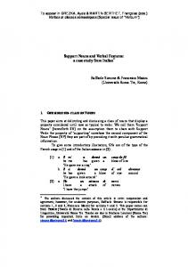


![Telephone Features User Guide - Avaya Support [PDF]](https://m.moam.info/img/260x300/telephone-features-user-guide-avaya-support-pdf_649bdf2c098a9e1c068b4666.jpg)


