Optimisation of non-integer order control parameters

Proceedings of ICAR 2003 The 11th International Conference on Advanced Robotics Coimbra, Portugal, June 30 - July 3, 2003

Optimisation of non-integer order control parameters for a robotic arm Duarte Val´ erio Jos´ e S´ a da Costa Technical University of Lisbon, Instituto Superior T´ecnico Department of Mechanical Engineering, GCAR Av. Rovisco Pais, 1049-001 Lisboa, Portugal {dvalerio;sadacosta}@dem.ist.utl.pt Abstract This paper describes the optimisation of control parameters for a two-link robotic arm. Hybrid position / force control had been implemented in the literature using non-integer order derivatives; genetic algorithms were now used for improving results. Significant improvements have been achieved for steady-state errors, maximum overshoots and settling times. Keywords: Non-integer order control; genetic algorithms; position / force hybrid control; optimisation; robot.

1

their improvement. Section 4 presents a comparison of results. Some conclusions are drawn in section 5.

2

The robot used in this paper is an arm with two degrees of motion consisting of two rigid links (with masses m1 and m2 , lengths r1 and r2 , moments of inertia J1m and J2m , and connected by joints with moments of inertia J1g and J2g ), leaning on a surface as seen in Figure 1. Its dynamic behaviour is given by [3, 5]

Introduction

τ

Controllers making use of non-integer order derivatives and integrals often achieve performance and robustness results superior to those obtained with conventional (integer order) controllers. Parameter tuning, however, is not always straightforward. Several methods have been proposed (see [7] for a survey) but have no application when the plant is highly nonlinear and complex. This is the case of hybrid position / force control of a robotic arm—the example addressed in this paper. A genetic algorithm was used for improving results found in the literature [3]. The paper is organised as follows. Section 2 presents the robotic arm. Section 3 introduces noninteger controllers and the genetic algorithm used for y

τ2 q1

q2

π/2 θ=π x

Figure 1: Robotic arm.

˙ + g(q) − JT (q)F(1) = H(q)¨ q + c(q, q)

H11 (q) = H12 (q) H21 (q) H22 (q) ˙ c1 (q, q)

= = = =

˙ c2 (q, q) =

(m1 + m2 )r12 + m2 r22 + 2m2 r1 r2 cos(q2 ) + J1m + J1g m2 r22 + m2 r1 r2 cos(q2 ) m2 r22 + m2 r1 r2 cos(q2 ) m2 r22 + J2m + J2g −m2 r1 r2 sin(q2 )q˙22 − 2m2 r1 r2 sin(q2 )q˙1 q˙2 m2 r1 r2 sin(q2 )q˙12

(2) (3) (4) (5) (6) (7)

g1 (q) = g(m1 r1 cos(q1 ) + m2 r1 cos(q1 ) + m2 r2 cos(q1 + q2 )) (8) g2 (q) = gm2 r2 cos(q1 + q2 ) (9) J11 (q) = −r1 sin(q1 ) + r2 sin(q1 + q2 ) (10) J21 (q) = r1 cos(q1 ) + r2 cos(q1 + q2 ) (11) J12 (q) = −r2 sin(q1 + q2 ) (12) J22 (q) = r2 cos(q1 + q2 ) (13)

yC xC

τ1

Robotic arm

where q = [ q1 q2 ]T is a 2 × 1 vector of joint coordinates, consisting of the angle made by the first link with the horizontal and the angle between the two links; τ = [ τ 1 τ 2 ]T is a 2 × 1 vector of actuator torques, consisting of the torques applied to each of the two joints of the robot; H(q) is a 2 × 2 inertia ma˙ is a 2×1 vector of centrifugal and Coriolis trix; c(q, q) terms; g(q) is a 2 × 1 vector of gravitational terms; J(q) is the 2 × 2 Jacobian matrix of the robot; and

387

m1 = 0.5 kg r1 = 1.0 m J1m = 1.0 kg m2 m2 = 6.25 kg r2 = 0.8 m J2m = 1.0 kg m2 2 J1g = 4.0 kg m M = 0.03 kg K = 400 N/m 2 J2g = 4.0 kg m B = 1.0 N s/m θ = π/2 rad Table 1: Robot and environment parameters.

Figure 2: Hybrid control scheme.

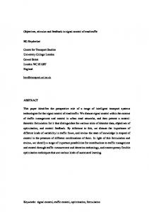
F is a 2 × 1 vector with the force exerted by the environment on the robot’s tip, which, the wall against which the robot leans being vertical and friction being neglected, will be modelled by · ¸ Mx ¨c + B x˙ c + Kxc F= (14) 0 Coordinate x will be force controlled and coordinate y will be position controlled; the hybrid control scheme is found in Figure 2 [2, 3]. The selection matrix S, the kinematic equations Λc (for finding the Cartesian coordinates (xc , yc ) from the joint coordinates (q1 , q2 )) and the Jacobian of these kinematic equations Jc are given by · ¸ 0 0 S = (15) 0 1  xc = r1 sin(θ − q1 )+    r2 sin(θ − q1 − q2 ) Λc : (16) y = r  c 1 cos(θ − q1 )+   r2 cos(θ − q1 − q2 ) Jc11 (q) = Jc12 (q) = Jc21 (q) = Jc22 (q) =

−r1 cos(θ − q1 ) − r2 cos(θ − q1 − q2 ) −r2 cos(θ − q1 − q2 ) r1 sin(θ − q1 ) + r2 sin(θ − q1 − q2 ) r2 sin(θ − q1 − q2 )

(17) (18) (19) (20)

This robot, with the parameters given in Table 1, was controlled in [3] using non-integer order derivatives. In that paper a reference test is used in which the robot begins at q1 = q2 = 15π/36 , without exerting force on the environment; a Fref = 1 N step at the force reference is applied when t = 0 , while the vertical position yc should remain constant, equal to its original position ycref .

3

Control

In this section non-integer order control of this plant and its tuning by a genetic algorithm are briefly exposed.

3.1 Non-integer control Non-integer order derivatives generalise usual, natn ural order derivatives Dn y(t) = d dty(t) . One of the n several existing definitions of non-integer order derivatives, which will be the most appropriate for what follows, is due to the work of Gr¨ unwald and Letnikoff, and is a generalisation of the usual definition of derivative, to wit, Dy(t) = lim

h→0

y(t) − y(t − h) h

(21)

that, for orders higher than 1, becomes, as may be easily proved by mathematical induction, µ ¶ Pn n k y(t − kh) k=0 (−1) k Dn y(t) = lim = h→0 hn µ ¶ P+∞ n k y(t − kh) k=0 (−1) k = lim (22) h→0 hn where the last equality holds since, given two natural numbers k > n, we have µ ¶ Γ(n + 1) n! n = = = 0 (23) k Γ(k + 1)Γ(n − k + 1) k!∞ So definition (22) may be generalised to define +∞ 1 X (−1)k Γ(v + 1)y(t − kh) , v∈< h→0 hv Γ(k + 1)Γ(v − k + 1) k=0 (24) Now the question arises of how to compute a noninteger order derivative of a time-sampled signal. Definition (24) of a derivative of arbitrary order is the basis for an approximation in which the time-step h will be approximated by the sampling time T , and the summation will be truncated after a finite number of terms n [4], resulting in " n # 1 X (−1)k Γ(v + 1)z −k v y(t) (25) D y(t) ≈ v T Γ(k + 1)Γ(v − k + 1)

Dv y(t) = lim

k=0

This formula might also have been obtained from a first-order backward finite difference (1 − z −1 )/T , which is a usual way of reckoning an approximation of a derivative from sampled values of a function. Raising the finite difference to a non-integer power v results in something which is not the ratio of two polynomials in z −1 . But performing a MacLaurin series

388

expansion we will obtain (as may be proved by mathematical induction) µ D

v

1 − z −1 T

¶v

y(t) ≈ y(t) = # "+∞ 1 X (−1)k Γ(v + 1)z −k y(t) (26) Tv Γ(k + 1)Γ(v − k + 1)

=

k=0

This formula, truncated after n terms, gives (25) again. Instead of a MacLaurin series expansion a continued fraction expansion can be used [7]. The result, after truncation, will be [6]  1 vz −1 − ≈ y(t)T −v 0; , , 1 1

Dv y(t) ≈ n −1

−1

i(i+v)z (2i−1)2i

1

,

− i(i−v)z 2i(2i+1) 1



(27)

i=1

Instead of using a first order finite difference for approximating derivatives, a usual formula for conversion between the continuous and the discrete do−1 mains, such as Tustin formula s ≈ T2 1−z 1+z −1 , may be used [4, 7]. The result will be [6] µ

µ ¶v 2 [1+ T  n X n i j −i X (−1) Γ(v + 1)Γ(i)2 z  (28) + Γ(v − j + 1)Γ(j)Γ(i − j + 1)Γ(j + 1) j=1 i=j Dv y(t) ≈

2 1 − z −1 T 1 + z −1

¶v

y(t) ≈ y(t)

3.2 Genetic algorithms Machado and Azenha [3] report that parameters in the first row of Table 2 were found by trial and error. Non-linear behaviour and complex relations between variables involved preclude the use of simple analytical methods; but refined means of trial and error may be employed. This is the case of derivative-free optimisation methods—such as genetic algorithms, simulated annealing or ant colonies—that rely not only on randomness to explore, as thoroughly as possible, the space of possible solutions, so that local minima may be avoided; but also try to improve, with each iteration, the best candidates found in the previous one [1]. In few words, a genetic algorithm is an iterative optimisation method that begins its first iteration with a randomly generated collection of possible solutions codified into binary numbers, which is called population, the members thereof being the individuals. The algorithm attempts to simulate the evolutionary principle of survival of the fittest. So, in each iteration, a performance index (or objective function) is evaluated for all individuals, and those found more fit are to have more chances to pass their characteristics onto another generation of individuals, which shall be evaluated at the next iteration. Generations after the first are obtained from the previous one by means such as mutation and crossover, which will be described below for the particular algorithm used in this instance. In the present case a starting point is given by the controllers of [3] and this eases the process of looking for solutions. The algorithm used is as follows: 1. Create a population consisting of 50 possible solutions. The first has the parameters of the controllers given in [3]; others are randomly obtained as follows:

if we use a MacLaurin series expansion and "

2 2v v 2 − i2 Dv y(t) ≈ ( )v 1; , 2i+1 1 T − z−1 − v − z−1

#n y(t) (29) i=1

• vF 1 and vF 2 are normally distributed with mean -1/5 and variance 5;

if we use a continued fraction expansion. There are still other ways of implementing noninteger controllers in the time domain [6]. Those above are the ones which performed better together with the optimisation method described below in subsection 3.2. Non-integer order controllers given in [3] for the plant described in section 2 are CF = [ GF 1 DvF 1

GF 2 DvF 2 ]T

(30)

CP = [ GP 1 DvP 1

T

(31)

GP 2 DvP 2 ]

• vP 1 and vP 2 are normally distributed with mean 1/2 and variance 5; • GF 1 is normally distributed with variance 250 and mean 103 T vF 1 +1/5 ; • GF 2 is normally distributed with variance 250 and mean 103 T vF 2 +1/5 ; • GP 1 is normally distributed with variance 25000 and mean 105 T vP 1 −1/2 ; • GP 2 is normally distributed with variance 25000 and mean 105 T vP 2 −1/2 .

implemented with the parameters given in the first row of Table 2. In what follows, n = 8 because a large n results in a larger steady-state error for the vertical position, in slightly larger overshoots for the force and in larger settling times: the value of n used here is a compromise with a smaller steady-state error for the force [6].

Those values are codified into a binary number as follows: • vF 1 is codified with 15 bits. 1 bit represents the sign, the other 14 the absolute value, multiplied by 1000. As a consequence, the resolution obtained is 0.001.

389

Original Set A Set B Set C Set D

GF 1 103 4.570 × 104 1.232 × 105 1.191 × 104 2.281 × 104

vF 1 -0.200 -0.750 -0.894 -0.556 -0.650

GF 2 103 1.741 × 103 0.704 × 103 2.075 × 104 2.024 × 103

vF 2 -0.200 -0.155 -0.187 -0.639 -0.292

GP 1 105 9.009 × 105 1.128 × 108 1.789 × 106 2.628 × 106

vP 1 0.500 0.180 -0.496 0.113 0.119

GP 2 105 1.381 × 105 9.479 × 104 8.146 × 104 4.326 × 104

vP 2 0.500 0.484 0.465 0.470 0.465

n 17 8 8 8 8

Formula (25) (25) (27) (28) (29)

Table 2: Control parameters. 1.4

• GF 1 is codified with 18 bits. Only positive integer values are possible (or, in other words, the resolution is 1). • vF 2 is codified with 15 bits, as vF 1 above. • GF 2 is codified with 18 bits, as GF 1 above. • vP 1 is codified with 15 bits, as vF 1 above. • GP 1 is codified with 18 bits, as GF 1 above. • vP 2 is codified with 15 bits, as vF 1 above. • GP 2 is codified with 18 bits, as GF 1 above.

Force (N)

1 0.8

0.2 0 0

I=

+

+

1000Sy2c

+

1000My2c

6. Eliminated individuals are replaced as follows: • One-half are replaced by mutations of the six remaining individuals. A random individual is chosen, and each binary digit thereof may undergo a change, with a probability of 4 %, so that the overall probability of no mutation is 0.5 %.

0.8

1

• One-fourth are replaced by a population created exactly as in point 1 (save that the total of created individuals is no longer 49, but one-fourth of the missing ones, as mentioned).

(36)

5. Eliminate all individuals in the population save those with the 6 best indexes of performance. (This policy of allowing the best performing individuals to live longer, not dying from one iteration to the next, is called elitism.)

0.4 0.6 Time (s)

• One-fourth are replaced by descendants of the six remaining individuals. Two random individuals are chosen. Each of the controllers GF 1 DvF 1 , GF 2 DvF 2 , GP 1 DvP 1 and GP 2 DvP 2 may be taken from one of those two, with equal probability. This mechanism is called crossover (in this case, three-point crossover, since each individual’s genome is cut into four by three cuts).

(32) (33) (34) (35)

4. If this is the 100th iteration, or if the best value of (36) did not change in the previous 10 iterations, stop the algorithm.

0.2

Figure 3: Control results: force.

These (percentage expressed) values were combined into a performance index. Several have been experimented; the one retained was 6MF2

BDC

0.4

3. Simulate control for all individuals in the population, implementing non-integer order derivatives with one of the formulas given in subsection 3.1. Determine maximum force overshoot, maximum position error, steady-state force error and stationary position error:

SF4

Original with n=8

0.6

2. Repeat the following steps until condition 4 is satisfied.

MF = 100% × (max(F ) − Fref )/Fref Myc = 100% × max(|yc − ycref |)/ycref SF = 100% × (F (1 s) − Fref )/Fref Syc = 100% × (yc (1 s) − ycref )/ycref

BADC

A

1.2

This algorithm deserves a few remarks. Firstly, it incorporates an unusual feature: randomly generated individuals, such as those of which the original population consists, appearing in every iteration—we may call this spontaneous generation. Secondly, parameter tuning (this refers to parameters as mutation probabilities, proportion of different kinds of new individuals when changing generation, number of elements in each generation) is—as is always the case with randomised search methods such as this one—a very important issue for which some trial and error is necessary. Selecting more general features of the algorithm (presence or absence of elitism, number of points for crossover. . . ) is also an arguable

390

matter without clear guidelines. Thirdly, the same may be said about the performance index—quantifying exactly how much we prefer overshoot to steady-state error is not always straightforward. Regarding this issue, it should be stressed that values of Syc and Myc are systematically very low. In spite of the 1000 weights in (36), the performance of the force control loop is always more important. This is quite reasonable since yc never deviates more than 2 mm from its reference. And it should be also stressed that performance indexes as the one chosen take no account of settling times or (even worst) highfrequency rippled responses. But settling times are no issue, since simulations are 1 s long and this is short enough to ensure that a good steady-state response has also a good settling time; and solutions presenting a high-frequency ripple may be rejected after the end of the algorithm. Fourthly, the accuracy of formulas given in subsection 3.1 for approximating non-integer order derivatives depends on the differentiation order v—and no formula is better than all others under all circumstances. As a consequence, depending on the formula used, the optimisation shall lead to different parameters for the controllers. Fifthly, a word is needed about why a genetic algorithm was preferred over other randomised search methods such as simulated annealing or ant colonies. A genetic algorithm has several features fit for solving this problem. It allows, by means of mutations, searching the vicinity of a good solution, varying its parameters slightly. Given two sets of good performing controllers, it allows, by means of crossover, experimenting combinations thereof. And it allows, by means both of mutations with severe effects and of randomly generated individuals appearing with each single iteration, exploring the space of solutions avoiding the trap of local minima. Now the simultaneous

1.366 CA

Reference Position (m)

1.3659 Original with n=8 BD

1.3658

1.3657 0

0.2

0.4 0.6 Time (s)

0.8

Figure 4: Control results: position.

1

existence of more than one possible solution is not found with simulating annealing, and ant colonies is a method that, though allowing application to continuous problems, is particularly fit for discrete ones, which is not the case, gains and differentiation (or integration) orders of the controllers being real. The same might be said about other optimisation methods. This does not mean, of course, that changing the method would preclude good (or even better. . . ) results.

4

Results

Figures 3 and 4, together with table 3, show the performance of the controller found in [3] (implemented, as explained above, with n = 8) together with that of the best controllers found with the genetic algorithm, given in table 2. Four sets of controllers are given, one for each of the formulas presented above for implementing non-integer order derivatives in the time domain. Improvements are clear over all components of the performance index and settling times. A few remarks ought to be made. Firstly, every attempt to reduce the force overshoot further, by increasing its weight in the performance index or by increasing its exponent, had as consequence a significant increase of the steady-state error. Secondly, the higher importance of the force control loop performance is clear from results, since position control, in certain cases, became worst, and nevertheless index I undergoes a clear decrease (this happened with controllers implemented with formulas using continued fractions). Thirdly, using parameters tuned with one formula for implementing non-integer order derivatives together with another formula was tried, but this does not (with very few exceptions) result in an improved behaviour. It seems clear that this optimisation is formula-dependent: as expected, the chosen formula conditions the control parameters obtained. Finally, these controllers do show an appreciable robustness. Figure 5 shows how the performance index changes when q1 and q2 vary (the position of the wall has been accordingly modified so that the simulation still begins with the robot at the desired position without exerting force on the environment). It was reckoned with the controllers of set B, but similar results might have been obtained with other sets. It shows that changing the initial conditions results in a poorer behaviour, but there is still a reasonably broad margin for which the control still remains stable. If variations of q1 and q2 are so large that behaviour becomes unacceptably poor or even unstable, other controllers will have to be obtained for the new conditions.

391

MF 1000Myc SF 1000Syc I F settling time (ms) yc settling time (ms)

Original (with n=8) 24.5% 5.1% -6.0% -2.2% 4959

Set A

Variation

Set B

Variation

Set C

Variation

Set D

Variation

12.3% 3.6% -2.5% -1.8% 959

-50% -29% -58% -18% -81%

7.0% 4.7% -2.4% -4.5% 370

-71% -8% -60% 105% -93%

9.4% 5.7% -4.0% -1.3% 815

-62% 12% -33% -41% -84%

6.8% 11.7% -2.9% -11.3% 620

-72% 129% -52% 414% -87%

362

177

-51%

178

-51%

181

-50%

217

-40%

576

334

-42%

223

-61%

429

-26%

343

-40%

Table 3: Control results. Settling times were computed with respect to the steady-state value, using the 2% criterion.

5

Conclusions

In this paper a genetic algorithm was successfully used for optimising non-integer control parameters of a robot subject to hybrid position / force control. Force and position overshoots, steady-state errors and settling times could be significantly reduced compared to the values obtained with parameters resulting from trial and error tuning, as published in the literature. The most obvious future work is repeating this optimisation with a model of a laboratory two-link robot (for which no trial and error pre-tuned non-integer order controllers exist, though), and then implementing it to ensure the validity of this method not only for this particular case but also as a general method of non-integer control parameter tuning fit for robotics. Further extensions would be applying the method to a robot with more than two links or to a flexible robot. In what concerns the method itself, other randomised search methods (such as simulated annealing or ant colonies) may be experimented instead of the genetic algorithm.

Acknowledgments This research was partially supported by programme POCTI, FCT, Minist´erio da Ciˆencia e do Ensino Superior, Portugal, grant number SFRH/BD/2875/2000, and ESF through the III Quadro Comunit´ ario de Apoio.

References [1] J.-S. R. Jang, “Derivative-free optimization,” in Neuro-fuzzy and soft computing, J.-S. R. Jang, C.T. Sun, E. Mizutani. Upper Saddle River: Prentice Hall, 1997, pp. 173-196. [2] O. Khatib, “A unified approach for motion and force control of robot manipulators: the operational space formulation,” IEEE Journal of robotics and automation, vol. 3, pp. 43-53, Feb. 1987. [3] J. Machado, A. Azenha, “Fractional-order hybrid control of robot manipulators,” in IEEE international conference on systems, man and cybernetics, 1998, pp. 788-793. [4] J. Machado, “Discrete-time fractional-order controllers,” Fractional calculus & applied analysis, vol. 4, pp. 47-66, Jan. 2001.

I

[5] L. Sciavicco, B. Siciliano, Modeling and control of robot manipulators. New York: McGraw-Hill, 1996, pp. 119-168. [6] D. Val´erio, J. S´a da Costa, “Digital implementation of non-integer control and its application to a two-link robotic arm,” in European Control Conference, 2003.

Figure 5: Control results: performance index as a function of initial conditions.

[7] B. Vinagre, Modelado y control de sistemas din´ amicos caracterizados por ecuaciones ´ıntegrodiferenciales de orden fraccional. Madrid: UNED, 2001.

392