water Article
Optimising Fuzzy Neural Network Architecture for Dissolved Oxygen Prediction and Risk Analysis Usman T. Khan 1 and Caterina Valeo 2, * 1 2
*
Department of Civil Engineering, Lassonde School of Engineering, York University, 4700 Keele St, Toronto, ON M3J 1P3, Canada;
[email protected] Department of Mechanical Engineering, University of Victoria, PO Box 1700 STN CSC, Victoria, BC V8P 5C2, Canada Correspondence:
[email protected]
Academic Editors: Yurui Fan and Jiangyong Hu Received: 30 March 2017; Accepted: 24 May 2017; Published: 28 May 2017
Abstract: A fuzzy neural network method is proposed to predict minimum daily dissolved oxygen concentration in the Bow River, in Calgary, Canada. Owing to the highly complex and uncertain physical system, a data-driven and fuzzy number based approach is preferred over traditional approaches. The inputs to the model are abiotic factors, namely water temperature and flow rate. An approach to select the optimum architecture of the neural network is proposed. The total uncertainty of the system is captured in the fuzzy numbers weights and biases of the neural network. Model predictions are compared to the traditional, non-fuzzy approach, which shows that the proposed method captures more low DO events. Model output is then used to quantify the risk of low DO for different conditions. Keywords: dissolved oxygen; water quality; artificial neural networks; fuzzy numbers; risk analysis; uncertainty
1. Introduction The dissolved oxygen (DO) concentration of a water body is the most fundamental indicator of overall aquatic ecosystem health [1–5]. Low DO concentrations can increase the risk of adverse effects to the aquatic environment. While the impact of long-term effects is largely unknown, low DO can have immediate and devastating effects on ecosystems [6]. Thus, DO is widely measured and modelled, and the identification and quantification of DO trends in rivers is of interest to water resource managers [7]. However, changes in watershed land-use due to urbanisation, the interaction of numerous factors, over a relatively small area and across different temporal scales means that DO is difficult to predict in urban areas [2,8]. Rapid changes in the urban environment (e.g., land-use changes or major flood events) means that the factors and regimes influencing DO in the riverine environment might also change rapidly. In Calgary, Alberta, Canada, the Bow River has experienced low DO conditions in recent years. The Bow River is extremely important for the region because it is a source of potable water, and is used for industrial, irrigation, fishing and recreational purposes [9,10]. Thus, maintaining a high water quality standard is extremely important. High sediment and nutrient loads, effluent from three wastewater treatment plants, and stormwater runoff have contributed to reducing the health of the Bow River. The City of Calgary is mandated to meet the requirements of the provincial surface water quality guidelines, which means maintaining DO concentrations above 5 mg/L (one-day minimum), and above 6.5 mg/L (seven-day average) [11]. Thus, in an effort to improve water quality and maintain high DO concentration the City has implemented several strategies to limit loadings such as the Total Loadings Management Plan and the Bow River Phosphorus Management Plan [12]. Water 2017, 9, 381; doi:10.3390/w9060381
www.mdpi.com/journal/water
Water 2017, 9, 381
2 of 24
As part of these plans, the City uses numerical modelling to predict the impact of different strategies within the watershed. However, the physical processes that govern the behaviour of DO in the aquatic environment are quite complex and poorly understood. The physically-based models that are typically used for DO prediction require the parameterisation of a several different variables, which can be unavailable, expensive and time consuming [7,13,14]. In addition to this, physically-based models cannot account for the rapid changes seen in the Bow River watershed, including two major floods in 2005 and 2013, new wastewater treatment plants that have come online, and the relocation of water quality monitoring stations further downstream. These factors highlight the fact that the uncertainty associated with the riverine ecosystem is high. Thus, DO predictions are extremely difficult and beset with uncertainty hindering water resource managers from making objective decisions. Thus, there is a need to create a numerical modelling method that can accurately predict DO concentration whilst accounting for the epistemic uncertainty in the system. 1.1. Data-Driven Models and ANN The City of Calgary currently uses a physically–based model: the Bow River Water Quality Model [15,16] to predict DO. This model suffers from many of the issues related to complexity and uncertainty that are discussed above. In response to this, recent research [5,14,17–19] has shown that data-driven models, particularly those that use abiotic factors as inputs have promising results to predict DO concentration. Examples of the abiotic factors used in these studies are water temperature, nutrient concentration, flow rate and solar radiation. These factors are commonly monitored at a high resolution in many jurisdictions including in Calgary. The advantage of using readily available data in these studies was twofold: first, it makes the system amenable to be modelled using data-driven models; and, second, if a suitable relationship between the abiotic factors and DO can be found, then changing the factors (e.g., increasing the discharge) could increase DO. Data-driven models are a class of numerical models based on generalized relationships between input and output datasets [20]. These models can characterize a system with limited assumptions and typically have a simple model structure. This means propagating the uncertainty through the model is easier. The use of data-driven models, such as artificial neural networks (ANNs), has been widespread in hydrology [21–23] including for DO prediction in rivers. Wen et al. [7] used an ANN to predict DO in a river in China using ion concentration as the predictors. Antanasijevi´c et al. [13] used ANNs to predict DO in a river in Serbia using a Monte Carlo approach to quantify the uncertainty in model predictions and temperature as a predictor. Chang et al. [24] also used ANNs coupled with hydrological factors (precipitation and discharge) to predict DO in a river in Taiwan. Singh et al. [25] used water quality parameters to predict DO and biochemical oxygen demand in a river in India. Other studies (e.g., [26,27]) have used regression methods to predict DO in rivers using water temperature as inputs. In general, these studies have demonstrated that data-driven models can provide a suitable format for predicting DO with lower complexity [13]. ANNs, popular type of data-driven model, are defined as a massively parallel distributed information processing system [7,23]. A commonly used type of ANN is called a Multi-Layer Perceptron (MLP) model which consists of three layers: an input layer, a hidden layer, and an output layer. Each layer consists of a number of neurons that each receives a signal (e.g., the input dataset), and, based on the strength of that signal (quantified by the model coefficients called weights and biases), emits an output. Thus, the final output layer is the synthesis and transformation of all the input signals from the input and hidden layers [28]. The number of neurons in the hidden layer is reflective of the complexity of the system being modelled; more neurons represent a more complex system [23]. The advantage of using ANNs is that complex systems can be modelled by ANNs without an explicit understanding of the physical phenomenon [13,29], making it an ideal candidate for DO prediction in riverine environments. However, recent surveys [30,31] on the state of the use of ANNs in the field indicate that the lack of uncertainty quantification is a major reason for the limited appeal of ANN by water resource managers. Uncertainty in ANN models stem from: (i) the choice of network
Water 2017, 9, 381
3 of 24
architecture, e.g., the number of hidden layers, the number of neurons in each hidden layer, and the transfer function between each layer; and the training algorithm used to quantify the weights and biases, including the fraction of data used for training, calibrating and testing; and (ii) the selection of the performance metric used for training which determines the value of the model coefficients. All of these factors can impact the final value of the model coefficients suggesting that a range of values for the weights and biases may be possible for the same dataset [31]. However, most ANN applications have a deterministic structure that does not quantify the uncertainty intervals corresponding to these predictions [32,33]. This means that end-users of these models may have excessive confidence in the forecasted values, and overestimate the applicability of the results [29]. However, as with all numerical models, the appropriate characterisation of uncertainty in a model is essential [34]. 1.2. Fuzzy Artificial Neural Networks for Risk Assessment Alvisi and Franchini [29] introduced a new method to train ANNs which used fuzzy numbers to quantify the total uncertainty in the weights, biases, and output of an ANN. Fuzzy numbers are an extension of fuzzy set theory [35] and express an uncertain or imprecise quantity. Fuzzy numbers are useful for dealing with uncertainties when data are limited or imprecise [36–39]. In this method, the model coefficients are defined to capture a predefined amount of observed data within different α-cut interval which are used to construct discretised fuzzy numbers. Khan and Valeo [19] further refined this technique by introducing an objective method to select the amount of data to be captured within each interval using the relationship between possibility and probability theory. An advantage of these approaches is that imprecise information (i.e., model output represented through the use of fuzzy numbers) can be effectively used to conduct risk analysis [40]. For example, the model output can be used to determine the risk of occurrence of low DO in the Bow River. However, given the overall preference of the general public and water resource managers for using probabilistic measures (rather than possibilistic or fuzzy measures), there is a need to convert the fuzzy number output of a fuzzy artificial neural network (FNN) to an equivalent probability for communicating risk and uncertainty. 1.3. Objectives Given the importance of DO concentration as an indicator of overall aquatic ecosystem health, there is a need to accurately model and predict DO in urban riverine environments. In this research, two separate methods are proposed to quantify the uncertainty in an ANN model used to predict DO. First, a transparent algorithm is developed to select the optimum network architecture to maximise model performance. In previous research using this dataset (e.g., [19]), an ad hoc trial and error approach was used in selecting the network architecture. In the current approach, the uncertainty introduced due to the use of data-driven models is carefully considered using the proposed algorithm to find the optimum network architecture. Secondly, a fuzzy number based ANN is implemented to quantify the total uncertainty of the model coefficients and output. Lastly, the application of the developed model is demonstrated by quantifying the risk of low DO in the Bow River using a new method. The results are used to create a tool for water resource managers to assess the risk of conditions that lead to low DO. The importance of the proposed approach is that it: (i) accounts for the complexity of the physical-system by using a data-driven approach; (ii) uses abiotic inputs since they are routinely collected and thus, a large dataset is available; and (iii) minimises the network architecture uncertainty and propagates the total uncertainty in the system through the use of fuzzy numbers. The present research uses crisp inputs as compared to fuzzy inputs in [19] for two practical reasons: (i) in some cases, high resolution data may not be available to construct fuzzy numbers using the algorithm introduced in [19], necessitating the use of observed crisp data (without input uncertainty quantification); and (ii) for the application component of this research, the inputs need to necessarily be crisp numbers in order to create a risk assessment tool for use by water resource managers. In other words, the proposed research will help managers identify the risk of low DO for any number of cases, using pre-selected crisp inputs.
Water 2017, 9, 381
4 of 24
Water 2017, 9, x FOR PEER REVIEW
4 of 25
2. Materials and Methods
2. Materials and Methods
2.1. Data Collection
2.1.The DataCity Collection of Calgary is located in the Bow River Basin (approximately 25,123 km2 in area) in
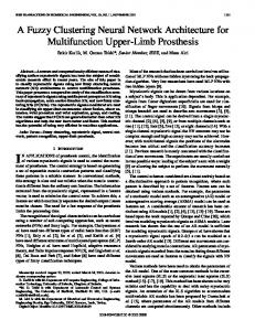
southern Alberta, Bow River 645 km long and (approximately averages a 0.4%25,123 slope over its area) lengthin[10]. The City ofCanada. Calgary The is located in theis Bow River Basin km2 in The headwaters of the river are located at Bow Lake, in the Rocky Mountains, from where it flows southern Alberta, Canada. The Bow River is 645 km long and averages a 0.4% slope over its length 2 south-easterly to Calgary (drainage of 7870 kmLake, ), meeting the Oldman Riverfrom andwhere eventually [10]. The headwaters of the river arearea located at Bow in the Rocky Mountains, it draining into Hudson Bay The river is supplied snowmelt from thethe Rocky Mountains, rainfall flows south-easterly to [9,41]. Calgary (drainage area of by 7870 km2), meeting Oldman River and eventually draining into from Hudson Bay [9,41]. The The River river has is supplied by snowmelt from theofRocky and runoff, and discharge groundwater. an average annual discharge 90 m3 /s, Mountains, rainfall discharge and an average widthand andrunoff, depthand of 100 m and from 1.5 m,groundwater. respectively The [42].River has an average annual an average widthofand depth of 100 m and 1.5 along m, respectively [42]. to measure discharge ofof 90Calgary m3/s, and The City samples a variety water quality parameters the Bow River The City of Calgary samples a variety of water quality parameters along the Bow River to the impacts of urbanisation. Real-time water quality monitoring systems are stationed at the upstream measure the impacts of urbanisation. Real-time water quality monitoring systems are stationed at 1). (at the Bearspaw reservoir) and downstream (at Highwood) ends of the City (as shown in Figure the upstream (at the Bearspaw reservoir) and downstream (at Highwood) ends of the City (as shown Comparing water quality data from the stations shows the direct impact of the urban area on the in Figure 1). Comparing water quality data from the stations shows the direct impact of the urban Bow River [18]: concentration at upstream site is generally high throughout the year, with little area on the Bow River [18]: concentration at upstream site is generally high throughout the year, diurnal variation [5,14,17], whereas the concentration downstream of the City limits is typically lower, with little diurnal variation [5,14,17], whereas the concentration downstream of the City limits is and experiences much higher fluctuations. The three wastewater treatment plants (shown in Figure 1) typically lower, and experiences much higher fluctuations. The three wastewater treatment plants are located upstream of this monitoring site, and are thought to be responsible, along with other (shown in Figure 1) are located upstream of this monitoring site, and are thought to be responsible, impacts of urbanisation, for degradation quality of atwater the site. along with other impacts ofthe urbanisation, for of thewater degradation quality at the site.
N
a b
c 0 2.5 5
10 km
d
e
f
Figure Anaerial aerialview viewCalgary, Calgary, Canada Canada showing (a)(a) Water Survey of Canada flowflow Figure 1. 1.An showingthe thelocations locationsof:of: Water Survey of Canada monitoring site “Bow River at Calgary (ID: 05BH004); (b) Bonnybrook; (c) Fish Creek; and (d) Pine monitoring site “Bow River at Calgary (ID: 05BH004); (b) Bonnybrook; (c) Fish Creek; and (d) Pine Creek wastewater treatment plants; and two water quality sampling sites: (e) Stier’s Ranch; and (f) Creek wastewater treatment plants; and two water quality sampling sites: (e) Stier’s Ranch; Highwood. and (f) Highwood.
For this research, nine years of DO concentration data were collected from the downstream For this years concentration data were fromstation the downstream station for research, the periodnine from 2004oftoDO 2012. From 2004 to 2007, thecollected monitoring was locatedstation at forPine the Creek periodand from 2004 to 2012. From 2004 to 2007, the monitoring station was located at Pine Creek sampled every 30 min (for 2004 and 2005), and every 15 min (for 2006 and 2007). In 2008 the station moved Stier’s it remained until2006 2011,and and2007). sampled datathe every and sampled everywas 30 min (forto2004 andRanch 2005),where and every 15 min (for In 2008 station hour (in 2008) andRanch every where 15 minit remained from thereuntil on. 2011, The site moved further was moved to Stier’s and was sampled data every downstream hour (in 2008)toand Highwood 2012there where sampled every 15 min. During this period atonumber of low every 15 min in from on.it The site was moved further downstream Highwood in DO 2012events where it were observed. The number of days where the observed DO was measured to be below 5 mg/L (the of sampled every 15 min. During this period a number of low DO events were observed. The number acute guideline) was 25 days in 2004, 1 day in 2005 and 25 days in 2006. The number of days with DO in days where the observed DO was measured to be below 5 mg/L (the acute guideline) was 25 days concentration below mg/Lin(the chronic guideline) waswith moreDO frequent with a below total of 2004, 1 day in 2005 and 6.5 25 days 2006. The number of days concentration 6.5184 mg/L occurrences: 41, 26, 70, 27, 5 and 15 days in 2004, 2005, 2006, 2007, 2008 and 2009, respectively. A YSI
Water 2017, 9, 381
5 of 24
(the chronic guideline) was more frequent with a total of 184 occurrences: 41, 26, 70, 27, 5 and 15 days in 2004, 2005, 2006, 2007, 2008 and 2009, respectively. A YSI sonde is used to monitor DO and the sonde is not accurate in freezing water [43], thus only data from the ice free period were considered, which is approximately from April to October for most years [19]. Since low DO events usually occur in the summer, the ice-free period dataset contains the dates that are of interest for low DO modelling. For this research, mean daily water temperature (T) and mean daily flow rate (Q) were selected as the abiotic input parameters for the FNN data-driven model. The reason for selecting these two variables was their use in previous studies in this river basin [5,14,17] which show that these variables are good predictors of DO concentration. The same YSI sonde used to sample DO concentration was used to collect T. The Water Survey of Canada site “Bow River at Calgary (ID: 05BH004 shown in Figure 1) was used to collect Q. These data are collected hourly throughout the year; data where considerable shift corrections are applied (usually due to ice conditions) were removed from the analysis. The mean annual water temperature ranged between 9.23 and 13.2 ◦ C, and the annual mean flow rate was between 75 and 146 m3 /s for the selected period. 2.2. ANN and Uncertainty Analysis For this research, a three layer, feedforward MLP type of ANN was selected to model minimum daily DO (the output) using Q and T as the inputs. Previous studies modelling minimum DO in the Bow River have also used a three-layer MLP feedforward network (see [17]). The type of ANN is extremely popular and thus, forms a reference for the basis of comparing ANN performance [28,29,44]. Two transfer functions were required: one between the input and hidden layer, which was selected as the hyperbolic tangent sigmoid function; and one between the hidden layer and output layer which was a pure linear function (following [7,23,29]). Similarly, the input and output data were pre-processed before training the network: the data were normalised so that all input and output data fell within the interval [−1, +1]. Model coefficients were calculated by minimising the mean squared error (MSE) between the modelled output and observed data (minimum DO). The Levenberg–Marquardt algorithm (LMA) was used as the training algorithm [45]. In LMA the error between the output and target is back-propagated through the model using a gradient method where the weights and biases are adjusted in the direction of maximum error reduction. To prevent over-fitting an early-stopping procedure is used [31,45] where the data are first split into three subsets (training, validation and testing). The training is terminated when the error on the validation subset increases from the previous iteration. 2.2.1. Network Architecture Two remaining factors relating to ANN architecture that need to be identified are: the number of neurons in the hidden layer (nH ), and the amount of data used for training, validation and testing (known as data-division) for the early-stopping procedure described above. There is no consistent method used in the literature for each of these factors [30,46,47]. Typically, an ad hoc, or trial-and-error method is used to select the number of neurons [17,23,29,31]. The number of neurons selected must balance the complexity and generalisation of the final model; too many neurons increase the complexity and hence the processing speed, while reducing the transparency of the model. Not enough neurons risk reducing model performance and forgoing the ability of modelling non-linear systems. Similarly, the issue of data-division, which can have significant impacts on final model structure, is also predominantly conducted in an ad hoc and trial-and-error basis [31]. Generally speaking, two broad methods are available: In the first, each subset should have data that are statistically similar, including similar patterns or trends. Conversely, a method can be selected where each subset is based on some physical property, such as grouping the subsets chronologically. In this research, we propose a coupled method to select the optimum nH and data-division for the ANN model described. The smallest number of neurons and the least amount of data for training is targeted. The first is to reduce computational effort. The second is to prevent the risk of over-fitting
Water 2017, 9, 381
6 of 24
to the training data, and to have a larger dataset for testing for more robust statistical inference of that dataset. First, the dataset is randomly split into a 50%:25%:25% ratio for training, validation and testing, respectively. For each subset, data are randomly sampled to group into each subset. Then, the network is trained using 1 to 20 neurons. This process is repeated 100 times to account for the different selection of randomly sampled data in each subset. This is because the random initialisation of the ANN can cause variability in overall model performance [44]. Thus, each iteration is different than the previous. The MSE for each test dataset is then calculated and compared, as well as the number of epochs for each model is measured. Epochs are the number of times each weight and bias is modified in the optimisation algorithm. The configuration that leads to the lowest MSE and the lowest number of epochs was collected. This process is then repeated by sequentially increasing the amount of data used for training (and thus, reducing the amount of data equally partitioned for validation and testing) by increments of 0.5% from 50% to 75%, conducting each iteration of this change 100 times. Using this process, the cases where the highest performance was measured can be listed, and the best combination (i.e., nH and amount of training data) can be objectively selected. In doing so, both the processing time (i.e., the number of epochs, the amount of training data and nH ) and the complexity (nH ) of the system is accounted for in the final model architecture. 2.2.2. Network Coefficients In the fuzzy ANN method developed by Alvisi and Franchini [29], the standard MLP model is modified to predict an interval rather than a single value for the weights, biases and outputs, corresponding to an α-cut interval (the lower and upper limits of a fuzzy set at a defined membership level α). This is repeated for several α-cut levels between 0 and 1 thus, building a discretised fuzzy number. The constraints are such that to find the upper and lower limits of each weight and bias to minimize the width of the predicted interval while capturing a predefined amount of data within each interval. Khan and Valeo [19] refined this method by utilising the relationship between possibility theory and probability theory, known as probability-possibility transformations (see [48–52]) for details). Khan and Valeo [19] adopted the transformation proposed by Dubois et al. [53], where the possibility is viewed as the upper envelope of the family of probability measures [50,54–56]. The same procedure is used in the present research to train the fuzzy ANN using deterministic inputs to construct fuzzy number coefficients (weights and biases) and outputs. Five intervals were selected corresponding to a membership level of 0, 0.2, 0.4, 0.6, and 0.8, with the deterministic result processed equivalent to a membership of 1. This FNN optimisation algorithm was implemented in MATLAB (version 2015a). The crisp results of the ANN (at a membership level, µ = 1) were conducted using the built-in MATLAB Neural Network Toolbox. Subsequent optimisation for the other intervals was conducted using a two-step approach: first the Shuffled Complex Evolution algorithm (commonly known as SCE-UA, [57]) was used to find an initial solution to the minimisation problem. Then, further refinement of the solution was conducted using the built-in MATLAB minimisation function fmincon. 2.3. Risk Analysis A major component of this research is to be able to use a trained fuzzy ANN model to predict the risk of low DO using abiotic inputs. However, communicating uncertainty, which can be done in a number of different ways, is an important, yet difficult task [58]. In this research defuzzification is used to convert the possibility of low DO (i.e., predicted minimum fuzzy DO to be below a given threshold) to a probability measure. The transformation is given as follows (following Khan and Valeo [18,19,42]): for any x in the support (the α-cut interval at µ = 0) of a fuzzy number [a, b], we have the corresponding
Water 2017, 9, 381
7 of 24
µ(x) and the paired value x' which also shares the same membership level. The value µ(x) is the sum of the cumulative probability distribution between [a, x] and [x', b], labelled AL and AR , respectively: µ(x) = AL + AR ,
(1)
where AL represents the cumulative probability between a and x which is assumed to equal the probability P(X < x), since the fuzzy number defines any values to less than a to be impossible (i.e., µ = 0). Given the fact that the fuzzy number is not symmetrical, the lengths of the two intervals [a, x] and [x', b] can be used to establish a relationship between AL and AR . Then, AL can be estimated as: AL = P(X < x) = µ(x)/{1 + [(b − x')/(x − a)]}.
(2)
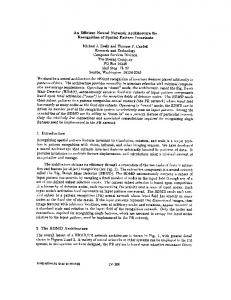
Thus, Equation (2), gives the probability that the predicted minimum DO for a given day is below the threshold value x. For example, if the lowest acceptable DO concentration of 5 mg/L [11] is selected as this threshold, then this transformation can be used to calculate the probability that daily minimum DO is below 5 mg/L. Similarly, the same principle can be used to map out all combinations of input values that lead to a risk of low DO (i.e., below 5 mg/L or any other threshold value). Once this is mapped out, combinations that lead to a major risk of low DO can be identified by water resource managers. The overall objective is to provide a simple tool to quantify the risk of low DO under selected T and Q conditions. For this research, the calibrated FNN model was used to predict minimum DO for various combinations of Q and T: where Q ranged between 40 m3 /s and 220 m3 /s (at 2 m3 /s intervals), and T ranged between 0 and 25 ◦ C (at 0.2 ◦ C intervals). For each prediction, the risk of low DO to be below either 5, 6.5 or 9.5 mg/L threshold was calculated using the previously described defuzzification technique. These intervals of Q and T were selected to reflect typical conditions in the Bow River. The thresholds correspond to the minimum acceptable DO concentration for the protection of aquatic life for 1-day (at 5 mg/L) [11], and for the protection of aquatic life in cold, freshwater for early-life stages (at 9.5 mg/L) and other-life stages (6.5 mg/L) [3]. 3. Results and Discussion 3.1. Network Architecture A three-layer, feedforward MLP network architecture was selected with 2 input variables and 1 output variable. A coupled method was used to determine the optimum nH and the percentage of data for each of the training, validation and testing subsets. Sample results of the proposed method are shown in Figure 2. Figure 2a shows the mean MSE (solid black line) of the test dataset for the initial 50%:25%:25% data-division scenario, with nH varying between 1 and 20 neurons. This simulation was repeated 100 times to account for the random selection of data and the upper and lower limits of MSE for each of these simulations are shown in grey. This figure demonstrates that the number of neurons did not have a noticeable impact on the MSE for this configuration. The most significant outcome of this process is that the variability (the difference between the upper and lower limits) of the performance seems to decrease after nH = 6 and increases again after nH = 12, with the lowest MSE at nH = 10. This result has two important implications: first, increasing the model complexity results in limited improvement of model performance, suggesting that a simpler model structure may be more suitable to describe the system. Second, the variability in performance indicates that the initial selection of data in each training subset can highly influence the performance of the test dataset, especially at the lower (i.e., nH < 6) and higher (i.e., nH > 12) ends of the spectrum of the proposed number of neurons. This suggests that an optimum selection of hidden neurons lies within this range (6 < nH < 12).
Water 2017, 9, 381
8 of 24
Water 2017, 9, x FOR PEER REVIEW
8 of 25 1000
4
50-25-25% data split
(b)
50-25-25% data split
(a)
800
3
Epochs for training
MSE of test dataset
3.5
2.5 2 1.5 1
600
400
200
0.5 0
5
10
15
0
20
5
Number of hidden neurons
300
Epochs for training
MSE of test dataset
20
n H = 10
(d)
n H = 10
(c)
3 2.5 2 1.5 1
250 200 150 100 50
0.5 0 50
15
350
4 3.5
10
Number of hidden neurons
55
60
65
Percent of training data
70
75
0 50
55
60
65
70
75
Percent of training data
Figure 2. Sample results thecoupled coupledmethod method to to determine determine the ofof neurons in in thethe Figure 2. Sample results ofofthe theoptimum optimumnumber number neurons hidden layer and percentage of data for training, validation and testing subsets; the mean (solid hidden layer and percentage of data for training, validation and testing subsets; the mean (solid black black line) and upper and lower limits (in grey) of: (a) the Mean Squared Error for the test dataset for line) and upper and lower limits (in grey) of: (a) the Mean Squared Error for the test dataset for each each number of hidden neurons; (b) the number of epochs for training; (c) the Mean Squared Error number of hidden neurons; (b) the number of epochs for training; (c) the Mean Squared Error for a for a range of training data size; and (d) the number of epochs for 10 hidden neurons. range of training data size; and (d) the number of epochs for 10 hidden neurons.
Figure 2b shows the change in the mean (solid black line) and the variability (in grey) of the Figureof2bepochs showsneeded the change inthe thenetwork mean (solid and the variability of the number to train for theblack initialline) data-division scenario, as(in nHgrey) increases number epochs needed trainvalue the network the ainitial data-division increases from of 1 to 20. While the to mean does notfor show notable change, the scenario, variabilityasofnHthe time needed forWhile training thevalue number of epochs) drastically as nvariability H increases of from to 5. needed This from 1 to 20. the(i.e., mean does not show a notabledecreases change, the the1time that a simpler modelofstructure requiredecreases more timeas tontrain, and the performance of these for means training (i.e., the number epochs)may drastically increases from 1 to 5. This means H simpler architectures (n H = 1 to 5) is more variable. This is likely because the initial dataset selection that a simpler model structure may require more time to train, and the performance of these simpler has a higher on the final model performance for less complex models. The lowest number of architectures (nimpact H = 1 to 5) is more variable. This is likely because the initial dataset selection has a mean epochs for this analysis occurred at nH = for 19, less withcomplex 26 epochs. However, thatnumber the variability higher impact on the final model performance models. Thenote lowest of mean of MSE at nH = 19 (in Figure 2a) is high, and that nH = 19 falls outside the range 6 < nH < 12, identified epochs for this analysis occurred at nH = 19, with 26 epochs. However, note that the variability of MSE above. at nH = 19 (in Figure 2a) is high, and that nH = 19 falls outside the range 6 < nH < 12, identified above. The impact of changing the amount of data used for training, validation and testing on the The impact of changing the amount of data used for training, validation and testing on the model model performance (MSE) was generally inconclusive as the amount of data used for training was performance (MSE) was generally inconclusive as the amount of data used for training was increased increased from 50% to 75% at 0.5% intervals. Figure 2c shows sample results for the nH = 10 scenario, from 50% to 75% 0.5%performing intervals. Figure 2c shows sample resultsmean for the nH = scenario, which was which was theatbest scenario, i.e., had the lowest MSE for10each data-division thescenarios best performing scenario, had lowest mean MSE for each data-division when compared toi.e., other nHthe values. However, the subplot illustrates that thescenarios MSE for when the compared to other n values. However, the subplot illustrates that the MSE for the test does H test dataset does not show a major trend as the amount of data for training is increaseddataset from the notinitial show 50%. a major trend as the amount of data for training is increased from the initial 50%. This means This means that for this scenario (nH = 10) increasing the amount of data used for training thathas forminimal this scenario (nH 10) increasing the amount of data has minimal impact on= model performance, indicating that used usingfor thetraining least amount of dataimpact for on model indicating usingavailable the leastfor amount of data training (and trainingperformance, (and thus having a higherthat fraction validating andfor testing) would bethus ideal.having Note a that fraction the meanavailable MSE values generally forwould all data-division scenarios the selected nH higher for were validating andhigher testing) be ideal. Note thatwhen the mean MSE values was betweenhigher 1 and 5for (follow the examplescenarios shown inwhen Figurethe 2a). were generally all data-division selected nH was between 1 and 5 (follow
the example shown in Figure 2a).
Water 2017, 9, 381
9 of 24
The number of epochs needed for training the network at different data-division scenarios was inconclusive. Figure 2d shows sample results for the nH = 10 case, which demonstrates that the mean and the variability of the number of epochs does not demonstrate a clear trend, as the amount of data used for training is increased. The significance of this analysis is that the amount of computational effort (or time) does not necessarily decrease as a larger fraction of data is used for training. Given this result, the least amount of training data (50%) is the preferred choice for the number of neurons that result in the lowest MSE, which is nH = 10 as described above. For the nH = 10 case, the overall mean number of epochs for each data-division scenario is low ranging between 24 and 40 epochs. Based on these results, nH = 10 with a 50%:25%:25% data-division was selected as the optimum architecture for this research. The fact that the mean and the variability of MSE was the lowest at nH = 10 makes it a preferred option over the nH = 19 case, which as a lower number of mean epochs but had higher variability in MSE. In other words, higher model performance was selected over model training speed (mean epochs at nH = 10 ranged between 9 and 122 for the 50%:25%:25% data-division scenario). Secondly no significant trend was seen as the amount of data used for training, validation and testing was altered, however lower MSE values were seen at nH = 10 compared to other at nH values. Thus, the option that guarantees the largest amount of independent data for validation and training is preferred. Given the fact that the mean MSE for the testing dataset does not show a significant change as the per cent of training data is increased from 50% to 75%, the initial 50%:25%:25% division is maintained as the final selection. The overall outcome of this component of this research was that that instead of using the typical trial-and-error based approach to selecting neural network architecture parameters, the proposed method can provide objective results. Specifically, systematically exploring different numbers of hidden layers and fraction of training data can help select a model with the highest performance, whilst accounting for the randomness in data selection. Once these neural network architecture parameters were identified, subsequent training of the FNN was completed. The results of the training and optimisation are presented in the next section. 3.2. Network Coefficients First, the network was trained at µ = 1 using the network structure outlined in the previous section. The crisp, abiotic inputs (Q and T) were used to estimate the values of each weight and bias in the network. This amounted to 20 weights (10 for each input) and 10 biases between the input and hidden layer, and 10 weights and 1 bias in the final layer. The MSE and the Nash–Sutcliffe model efficiency coefficient (NSE; [59]) for the training, validation and testing scenarios for the µ = 1 case are shown in Table 1 below. Table 1. Mean Squared Error and the Nash–Sutcliffe model Efficiency coefficient for the neural network at a membership level equal to 1.
Train Validation Test
MSE (mg/L)2
NSE
1.04 1.22 1.42
0.59 0.61 0.51
The MSE for each dataset is low, approximately between 10% and 18% of the mean annual minimum DO seen in the Bow River for the study period. The NSE values are greater than 0.5 for each subset, which is higher than NSE values for most water quality parameters (when modelled daily) reported in the literature [60] and is considered “satisfactory” using the ranking system proposed by Moriasi et al. [60]. These two model performance metrics highlight that predicting minimum DO using abiotic inputs and a data-driven approach is an effective technique. Note that compared to results reported in [19], the present modelling approach (with the optimised network architecture) produces similar performance metrics (i.e., “satisfactory”). However, note that in the present case
Water 2017, 9, 381
10 of 24
the network architecture selection is selected using an explicit and transparent algorithm, rather than in an ad hoc manner as in [19]. While both methods use the same dataset, the network architecture (number of neurons) is different for both methods, resulting in minor discrepancies between the model performance metrics. Additionally, some results in [19] are derived from fuzzy inputs rather than crisp inputs (as is the case in the present work). Additional advantages of the proposed approach are seen when the fuzzy component of the results are analysed. Once the crisp network was trained, a top down approach was taken to train the remaining intervals, starting at µ = 0.8 where 20% of the observations should be captured within the corresponding predicted output interval, and continuing to µ = 0 where 99.5% of the observations should be captured within the predicted output intervals. Each set of optimisation (both the SCE-UA and fmincon algorithms) for each of the five remaining membership levels (µ = 0, 0.2, 0.4, 0.6 and 0.8) took approximately 2 h using a 2.40 GHz Intel® Xeon microprocessor (with 4 GB RAM). The results of this optimisation are summarised in Table 2, which shows the amount of data captured within the resulting α-cut intervals after each optimisation. Table 2. Percentage of data (%) captured within each fuzzy interval for the Fuzzy Neural Network model. µ
Train
Validation
Test
1.00 0.80 0.60 0.40 0.20 0.00
– 20.02 40.05 60.07 80.10 99.51
– 16.10 34.63 52.44 80.00 98.78
– 15.85 33.41 52.44 80.24 99.02
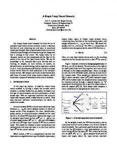
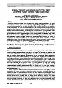
For the training dataset, the coupled algorithm was able to capture the exact amount of data it was required to. Similar results can be seen for the validation and testing datasets, where the amount of data captured are close to the constraints posed. For the two independent datasets, the amount of coverage decreases (i.e., lower performance) as the membership level increases, which is unavoidable when the width of the uncertainty bands decrease. Similar results were seen for the testing dataset in [29]. These results are similar to those published in [19] for both the fuzzy and crisp input case, with the only marked differences are: at the µ = 0.4 level where the present model captures a lower percentage of data than the crisp case in the previous method; and at the µ = 0.2 and 0.8 levels where the present model captures data closer to the assigned constraints as compared to the fuzzy inputs case in [19]. The result of this optimisation was the calibrated values of the fuzzy weights and biases; sample membership functions for four weights and biases are shown in Figure 3. The figure illustrates that the shapes of all membership functions were convex, a consequence of the top-down calibration approach, where the interval at lower membership levels is constrained to include the entire interval at higher membership levels. In other words, since lower membership levels include a higher amount of data, the corresponding interval to that level is wider than at higher membership levels. Furthermore, since the crisp network was used at µ = 1, there is at least one element in each fuzzy number with µ = 1, meaning that each weight and bias is a normal fuzzy set.
Water 2017, 9, 381
11 of 24
Water 2017, 9, x FOR PEER REVIEW
11 of 25
1
1
0.8
0.8
0.6
0.6
0.4
0.4
0.2
0.2
0
2
2.2
2.4
2.6
2.8
Weight # 10 : between input and hidden layer
0 -1.8
1
1
0.8
0.8
0.6
0.6
0.4
0.4
0.2
0.2
0 0.4
0.42
0.44
0.46
0.48
0.5
Weight # 2 : between hidden and output layer
-1.6
-1.4
-1.2
-1
Bias # 4 : between input and hidden layer
0 0.12
0.14
0.16
0.18
0.2
Bias # 1 : between hidden and output layer
Figure 3. Sample resultsofofthe theFuzzy FuzzyNeural Neural Network Network optimisation toto estimate thethe fuzzy Figure 3. Sample results optimisationalgorithm algorithm estimate fuzzy number values of selected weights and biases in the FNN model. number values of selected weights and biases in the FNN model.
The membership functions of the weights and biases are assumed to be piecewise linear
The membership functions of the and This biases are assumed to be α-cut piecewise linear following the assumption made in weights [5,14,19,29]. means that enough levels needfollowing to be theselected assumption made in [5,14,19,29]. This means that enough α-cut levels need to be selected to completely define the shape of the membership functions. In this research six levels were to completely define thespan, shape of to thegive membership functions. In this research levels were selected selected to equally and a full spectrum of possibilities, betweensix 0 and 1. Overall, the to equally and to give a full spectrum of demonstrate possibilities,that between and 1. Overall, theselected results of results ofspan, the weights and biases in the figure indeed0enough levels were define the of in thethe membership function. If that a smaller number of levels selected, e.g., thetoweights andshape biases figure demonstrate indeed enough levelswere were selected to two define levels, one at μ = 0 and one at μ = 1, the fuzzy number collapses to a triangular fuzzy number. This the shape of the membership function. If a smaller number of levels were selected, e.g., two levels, a full description of athe uncertainty andnumber. how it changes in of onetype at µof= fuzzy 0 and number one at µdoes = 1, not the provide fuzzy number collapses to triangular fuzzy This type relation to the membership level. Thus, intermediate intervals are necessary and the results fuzzy number does not provide a full description of the uncertainty and how it changes in relation to theThus, functions are in fact not triangular shapedand functions and not necessarily thedemonstrate membershipthat level. intermediate intervals are necessary the results demonstrate that symmetric about the modal value (at μ = 1). A consequence of this is that the decrease in sizeabout of thethe the functions are in fact not triangular shaped functions and not necessarily symmetric intervals does not follow a linear relationship with the membership level. Similarly, a higher number modal value (at µ = 1). A consequence of this is that the decrease in size of the intervals does not of intervals than the six selected for this research could be used, e.g., 100 intervals, equally spaced follow a linear relationship with the membership level. Similarly, a higher number of intervals than between 0 and 1. The risk in selecting many intervals is that as the membership level increases the six selected for this research could be used, e.g., 100 intervals, equally spaced between 0 and 1. (closer to 1) the intervals become narrower as a consequence of convexity. This will result in Thenumerous risk in selecting many intervals is that as the membership level increases (closer to 1) the intervals closely spaced intervals, with essentially equal upper and lower bounds, making the extra become narrower as a consequence of convexity.inThis will result in numerous closelyforspaced information redundant. This is demonstrated the sample membership functions WIH =intervals, 10 in with essentially upperthe and lowerofbounds, making the extra information redundant. This is Figure 3, whereequal increasing number membership levels between 0.4 and 1.0 would not improve demonstrated in the sample membership functions for WIH = 10 in Figure 3, where increasing the shape or description of the membership function. This is because the existing intervals arethe number of quite membership between 0.4 and 1.0 would not improve the shape or description of the already narrow. levels Defining more uncertainty bands between the existing levels would not add membership This is because thethe existing intervals are calculated. already quite narrow. Defining more more detailfunction. but would merely replicate information already Tablebands 2 andbetween Figure 3 the demonstrate the overall success of the proposed approach calibrate an uncertainty existing levels would not add more detail but would to merely replicate model. Whereas in many fuzzy set applications the membership function is not defined or theFNN information already calculated. selected on a consistent, transparent or objective method is selected Table 2based and Figure 3 demonstrate the overall success of the[30,46,47], proposedorapproach toarbitrarily calibrate an (as model. noted inWhereas [29]), the in method this research the is based on possibility theoryisand FNN manyproposed fuzzy setinapplications membership function not provides defined or an objective method to create membership functions. The results of the process show the selected based on a consistent, transparent or objective method [30,46,47], or is selected that arbitrarily method is capable in creating fuzzy number weights and biases that are convex and normal, and (as noted in [29]), the method proposed in this research is based on possibility theory and provides an capture the required percentage of data within each interval. objective method to create membership functions. The results of the process show that the method
Water 2017, 9, 381
12 of 24
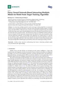
is capable in creating fuzzy number weights and biases that are convex and normal, and capture the Water 2017, 9, x FOR PEER REVIEW 12 of 25 required percentage of data within each interval. Figure 4 shows the results of observed versus crisp predictions (black dots) and fuzzy predictions Figure 4 shows the results of observed versus crisp predictions (black dots) and fuzzy predictions (black line) of minimum DO at the membership level µ = 0 for the three different data subsets. (black line) of minimum DO at the membership level μ = 0 for the three different data subsets. The The figure illustrates that nearly all (i.e., ~99.5%) of the observations fall within the α-cut interval figure illustrates that nearly all (i.e., ~99.5%) of the observations fall within the α-cut interval defined at defined at µ = 0 since the black dots are enveloped by the grey high-low lines of the fuzzy interval. μ = 0 since the black dots are enveloped by the grey high-low lines of the fuzzy interval. The figure also Thedemonstrates figure also demonstrates advantage FNN overwhile a simple some of the crisp the advantage the of the FNN overofa the simple ANN: someANN: of the while crisp predictions veer predictions veer from the 1:1 line (especially at low DO, defined tomg/L be less thannearly-all 6.5 mg/L(i.e., here), away from theaway 1:1 line (especially at low DO, defined to be less than 6.5 here), nearly-all (i.e., ~99.5%) of the fuzzy predictions intersect the 1:1 line. This also illustrates that the NSE ~99.5%) of the fuzzy predictions intersect the 1:1 line. This also illustrates that the NSE values reported values reported in Table 1 (which were calculated for the crisp case at µ = 1 only) are not representative in Table 1 (which were calculated for the crisp case at μ = 1 only) are not representative of the NSE of the NSE of number the fuzzy number predictions, and there is a need to developperformance an equivalent values ofvalues the fuzzy predictions, and that there is athat need to develop an equivalent performance metric whencrisp comparing crisp to observations to predictions. fuzzy number predictions. metric when comparing observations fuzzy number Training dataset
Validation dataset 15
15
10
10
5
5
0 0
5
10
15
Observed minimum DO, mg/L
0
0
5
10
15
Observed minimum DO, mg/L
Testing dataset Crisp predictions Predicted = 0 interval 1:1 line 6.5 mg/L limit
15
10
5
0
0
5
10
15
Observed minimum DO, mg/L Figure 4. A comparison of the observed and predicted crisp (black dots) and fuzzy intervals at μ = 0
Figure 4. A comparison of the observed and predicted crisp (black dots) and fuzzy intervals at (grey lines) for minimum Dissolved Oxygen in the Bow River for the training, validation and testing µ = 0 (grey lines) for minimum Dissolved Oxygen in the Bow River for the training, validation and datasets. testing datasets.
Lastly, the figure demonstrates the superiority of the FNN to be able to predict more of the low Lastly, the figure demonstrates the superiority therange FNN(at toDO be able predict more of theinlow DO events compared to the crisp method. The low of DO = 6.5to mg/L) is highlighted DOFigure events compared to the crisp method. The low DO range (at DO = 6.5 mg/L) is highlighted 4, and it is apparent that within this window both models tend to over predict minimum DO in as they fallitabove the 1:1 line. However, the fuzzy intervals lines) by the FNN Figure 4, and is apparent that within this window both models (grey tend to overpredicted predict minimum DO as intersect the 1:1 line for the majority of low DO events, and hence predict some possibility (even if it
Water 2017, 9, 381
13 of 24
Minimum Daily DO, mg/L
Minimum Daily DO, mg/L
they fall above the 1:1 line. However, the fuzzy intervals (grey lines) predicted by the FNN intersect Water 2017, 9, x FOR PEER REVIEW 13 of 25 the 1:1 line for the majority of low DO events, and hence predict some possibility (even if it is a low probability) at any µ ofat the low events, whereas crisp do predict any possibility at all. Thus, is a low probability) any μ DO of the low DO events,the whereas thenot crisp do not predict any possibility generally speaking the ability of the FNN to capture 99.5%toofcapture the data99.5% within intervals at all. Thus, generally speaking the ability of the FNN of its thepredicted data within its guarantees that most of the low DO events are successfully predicted. This is a major improvement predicted intervals guarantees that most of the low DO events are successfully predicted. This is over a major improvement over conventional used to predict Comparing Figure 4into[19] conventional methods used to predict lowmethods DO. Comparing Figure low 4 to DO. similar results reported similar results in [19] approach demonstrate thatpresent the proposed approach in the present has demonstrate thatreported the proposed in the research has improved modelresearch performance. improved model performance. Specifically, the predicted intervals at μ = 0 are centred on the output Specifically, the predicted intervals at µ = 0 are centred on the output rather than skewed. An outcome rather thanthere skewed. outcome of of this“false is that there (i.e., are apredicting lower number of “false (i.e., of this is that are aAn lower number alarms” low DO event alarms” when observed predicting low DO event when observed DO was not low) compared to [19]. This is discussed in DO was not low) compared to [19]. This is discussed in more detail below. This suggests that by using detailalgorithm below. This that low by using an optimised algorithmatfor network, DO an more optimised for suggests the network, DO prediction is improved, thethe expense of alow predicting prediction is improved, at the expense of a predicting high DO events (i.e., the upper limit of the high DO events (i.e., the upper limit of the predicted intervals). However, high DO values are of less predicted intervals). However, high DO values are of less interest and importance to most operators. interest and importance to most operators. Figures 5 and 6 show trend plots of observed minimum Figures 5 and 6 show trend plots of observed minimum DO and predicted fuzzy minimum DO for DO and predicted fuzzy minimum DO for the years 2004, 2006, 2007 and 2010. These particular years the years 2004, 2006, 2007 and 2010. These particular years were selected due to the high number of were selected due to the high number of low DO occurrences in each year, and, thus, are intended low DO occurrences in each year, and, thus, are intended to highlight the utility of the proposed to highlight the utility of the method. Note that,50% for of each approximately method. Note that, for eachproposed year shown, approximately theyear datashown, constitute training data,50% of the data constitute training data, while the other 50% constitute a combination of validation while the other 50% constitute a combination of validation and testing data. However, for clarity,and testing data. However, for clarity, this difference is not explicitly shown in these figures. this difference is not explicitly shown in these figures.
Figure 5. Time-series comparison ofobservations the observations and Fuzzy Network minimum Figure 5. Time-series comparison of the and Fuzzy NeuralNeural Network minimum Dissolved Dissolved Oxygen for 2004 and 2006. Oxygen for 2004 and 2006.
Water 2017, 9, 381
14 of 24 14 of 25
Minimum Daily DO, mg/L
Minimum Daily DO, mg/L
Water 2017, 9, x FOR PEER REVIEW
Figure 6. Time-series comparison of the observations and Fuzzy Neural Network minimum
Figure 6. Time-series comparison of the observations and Fuzzy Neural Network minimum Dissolved Dissolved Oxygen for 2007 and 2010. Oxygen for 2007 and 2010.
The most number of days where minimum daily DO was below the 5 mg/L guideline was The most number of days where minimum dailyThe DOyear was2007 below 5 mg/L was observed in 2004 and 2006, with 25 days in each year. had the the third mostguideline (after 2006 and 2004, respectively) number of days below the 6.5 mg/L guideline, with 27 days. Lastly, 2010 had observed in 2004 and 2006, with 25 days in each year. The year 2007 had the third most (after 2006 and therespectively) second most number guideline withwith 180 27 days (after 2007 which hadthe 2004, number of ofdays daysbelow belowthe the9.5 6.5mg/L mg/L guideline, days. Lastly, 2010 had 182) most belownumber the guideline. four yearsguideline collectively represent years with the lowest second of daysThus, belowthese the 9.5 mg/L with 180 daysthe (after 2007 which had 182) minimum daily DOThus, during the four study period. It is noteworthy that though minimum was below the guideline. these years collectively represent theeven years with the lowestDO minimum observed to be below 5 mg/L on several occasions in 2004 and 2006, the DO was below on 9.5 mg/L daily DO during the study period. It is noteworthy that even though minimum DO was observed to only 107 and 164 respectively, for2004 theseand years. In the contrast, in 2007 and no observations be below 5 mg/L ondays, several occasions in 2006, DO was below on2010, 9.5 mg/L only 107 and below 5 mg/L were seen, however 182 and 180 days, respectively, below the 9.5 mg/L were seen for 164 days, respectively, for these years. In contrast, in 2007 and 2010, no observations below 5 mg/L those years. This indicates that even if no observations of DO < 5 mg/L are seen, it is not a good were seen, however 182 and 180 days, respectively, below the 9.5 mg/L were seen for those years. This indicator of a healthy ecosystem, since the overall mean DO of the year might be low (e.g., a majority indicates that even if no observations of DO < 5 mg/L are seen, it is not a good indicator of a healthy of days below the 9.5 mg/L). The implication of this is that only using one guideline is not a good ecosystem, since the overall mean DO of the year might be low (e.g., a majority of days below the indicator of overall aquatic ecosystem health. 9.5 mg/L). The implication this is that only using guidelinemembership is not a good indicator overall L or In Figures 5 and 6, theofpredicted minimum DO one at equivalent levels (e.g., 0of 0 R) aquatic ecosystem health. at different times steps are joined together creating bands representative of the predicted fuzzy In Figures 5 and 6,atthe predicted at equivalentLmembership levels (e.g., 0L orand 0R ) at numbers calculated each time step.minimum Note thatDO the superscripts and R define the lower bound different steps areinterval joined at together creatinglevel bands representative of doing the predicted fuzzy numbers upper times bounds of the a membership of 0, respectively. In so, it is apparent that calculated at each values time step. Note that L and R 2006, define theand lower bound and upper all the observed fall within the μthe = 0superscripts interval for the years 2007 2010, and nearly all observations in 2004. This in 2004 is of because the per centIn of doing data included the μ = 0 all bounds of the interval at a difference membership level 0, respectively. so, it iswithin apparent that was selected to be 99.5% rather than for 100% prevent the optimisation theinterval observed values fall within the µ = 0 interval thetoyears 2006,over-fitting; 2007 and 2010, and nearly all algorithm was designed eliminatein the outliers first to the minimise theof predicted interval. The low observations in 2004. This to difference 2004 is because per cent data included within theDO µ=0 valueswas in 2004 are the lowest of the study period, thus areover-fitting; not capturedthe by optimisation the FNN. interval selected to be 99.5% rather than 100%and to prevent algorithm The width of each the band corresponds to the amount of uncertainty withvalues each in was designed to eliminate outliers first to minimise the predicted interval.associated The low DO membership level, for example, the bands are the widest at μ = 0, meaning the results have the most 2004 are the lowest of the study period, and thus are not captured by the FNN. vagueness associated with it. Narrower band are seen as the membership level increases until μ = 1, The width of each band corresponds to the amount of uncertainty associated with each which gives crisp results. This reflects the decrease in vagueness, increase in credibility, or less membership level, for example, the bands are the widest at µ = 0, meaning the results have the uncertainty of the predicted value. In each of the years shown, note that the observations fall closer most vagueness associated with it. Narrower band are seen as the membership level increases until to the higher credibility bands, except for some of the low DO events. This means that the low DO µ = 1, which gives crisp results. This reflects the decrease in vagueness, increase in credibility, or events are mostly captured with less certainty or credibility (typically between the 0L and 0.2L levels)
less uncertainty of the predicted value. In each of the years shown, note that the observations fall
Water 2017, 9, 381
15 of 24
Minimum Daily DO, mg/L
Minimum Daily DO, mg/L
Minimum Daily DO, mg/L
Minimum Daily DO, mg/L
closer to the higher credibility bands, except for some of the low DO events. This means that the low DO events are mostly captured with less certainty or credibility (typically between the 0L and 0.2L levels) compared to the higher DO events. However, it should be noted that compared to a crisp ANN, Water 2017, 9, x FOR provides PEER REVIEW 15 of 25 a crisp the proposed method some possibility of low DO, whereas the former only predicts result without a possibility of low DO. Thus, the ability to capture the full array of minimum DO compared to the higher DO events. However, it should be noted that compared to a crisp ANN, the within different is an advantaged of the method existing methods. proposed intervals method provides some possibility of proposed low DO, whereas theover former only predicts a crisp Results 2004 show thatofminimum DO the decreases rapidly in late and continuing resultfrom without a possibility low DO. Thus, ability to capturestarting the full array of June minimum DO within different intervals is an advantaged of the proposed method over existing methods. until late July, followed by a few days of missing data and near-zero measurements, before increasing Results from 2004 show that minimum DO decreases rapidlyinstarting in 7. lateThe Junereason and continuing to higher DO concentration. Details of this trend are shown Figure for this rapid until late July, followed by a few days of missing data and near-zero measurements, before increasing decrease is unclear and may be an issue with the monitoring device. However, it demonstrates that to higher DO concentration. Details of this trend are shown in Figure 7. The reason for this rapid the efficacy of data-driven is dependent on the quality of the data. One of the advantages decrease is unclear andmethods may be an issue with the monitoring device. However, it demonstrates that the of the proposed method is that while it is able to capture nearly all of the observations efficacy of data-driven methods is dependent on the quality of the data. One of the advantages of(including the method that whileband it is able nearly all of the observations outliers)proposed within the leastiscertainty (at µto=capture 0), other observations are mostly(including capturedoutliers) within higher within the least certainty band (at μ = 0), other observations are mostly captured within higher certainty bands (µ > 0). As the data length increases (i.e., the addition of more data and the FNN is certainty bands (μ > 0). As the data length increases (i.e., the addition of more data and the FNN is updated), the number of outliers included with the µ = 0 band will decrease because the optimisation updated), the number of outliers included with the μ = 0 band will decrease because the optimisation algorithm searches for the smallest width of the interval whilst including 99.5% of the data. Thus, with algorithm searches for the smallest width of the interval whilst including 99.5% of the data. Thus, with more data, the 0.5% in in the willbebethe the type of outliers seen more data, the not 0.5%included not included theinterval interval will type of outliers seen in 2004.in 2004.
Figure 7. Detailed view of time series for minimum observed Dissolved Oxygen and predicted fuzzy Figure 7. Detailed view of time series for minimum observed Dissolved Oxygen and predicted Dissolved Oxygen for 2004, 2006, 2007 and 2010, corresponding to days with low Dissolved Oxygen fuzzy Dissolved Oxygen for 2004, 2006, 2007 and 2010, corresponding to days with low Dissolved events. Oxygen events.
The time series plot for 2006 shows that all the observations fall within the predicted intervals. majority the for 25 low DO (i.e., less mg/L) occur starting mid-July continuing TheThe time seriesofplot 2006 shows thatthan all 5the observations fallinwithin theand predicted intervals. occasionally until mid-September. Unlike in 2004, all of these low DO events are captured within The majority of the 25 low DO (i.e., less than 5 mg/L) occur starting in mid-July and continuing both the μ = 0.2 and 0 intervals. This suggests that the model predicts these low DO events with occasionally mid-September. Unlike in 2004, all ofofthese low events areplotted captured within both more until credibility than in the 2004 case. Details of some the low DODO events are also in Figure the µ = 70.2 and 0 intervals. suggests the DO model predicts thesebetween low DOμ events (for September). This This plot shows that that the low events are captured = 0 andwith 0.2 more intervals. Even the membership trend profile of plotted the observed credibility than in thethough 2004 case. Details of level someisoflow, thethe lowgeneral DO events are also in Figure 7 minimum This daily plot DO isshows captured by the the modelled results. are captured between µ = 0 and 0.2 intervals. (for September). that low DO events Figure 6 illustrates the time series predictions for 2007, and it clearly demonstrates that most of Even though the membership level is low, the general trend profile of the observed minimum daily the observations are captured at higher membership levels, unlike the 2004 and 2006 examples, i.e., DO is captured by the modelled results. only a limited number of observations are seen between the μ = 0 and 0.2 intervals for the entire year. Figure 6 illustrates theout time series predictions for 2007, and clearly that most In addition to this, 26 of the 27 low DO observations (in this caseitbelow 6.5demonstrates mg/L) for this year of the observations are captured at higher membership levels, unlike the 2004 and 2006 examples, i.e., only a limited number of observations are seen between the µ = 0 and 0.2 intervals for the entire
Water 2017, 9, 381
16 of 24
year. In addition to this, 26 out of the 27 low DO observations (in this case below 6.5 mg/L) for this year are captured within the predicted membership levels (between µ = 0 and 0.2). Figure 7 shows details of a low DO period in 2007 in July and August, which shows that the observations are evenly scattered around the µ = 1 line. The trend plot for 2010 is shown Figure 6 and it is clear that nearly all observations for the year are below 10 mg/L, and about 87% of all observations are below the 9.5 mg/L guideline. As with the 2007 case, the bulk of the observations are captured within high credibility intervals, owing to the lack of extremely low DO (i.e., below 6.5 or 5 mg/L). The trend plot illustrates that the FNN generally reproduces the overall trend of observed minimum DO. This can be seen in a period in early May where DO falls from a high of 10 mg/L to a low of 7 mg/L, and all the predicted intervals replicate the trend. This is an indication that the two abiotic input parameters are suitable parameters for predicting minimum DO in this urbanised watershed. Figure 7 shows details of a low DO (below 9.5 mg/L) event in 2010 in late July through late August. The bulk of low DO events are captured between the µ = 0.6 and 0.2 intervals—demonstrating that these values are predicted with higher credibility than the low DO cases (