Optimization Using Chaotic Neural Network and Its Application to Lighting Design by
Ryuichi
Nanba1,
Mikio
Hasegawa2,
1Department
Tomoyuki Nishita1 and Kazuyuki Aihara1, 3
of Complexity Science and Engineering
Graduate School of Frontier Sciences The University of Tokyo 7-3-1 Hongo, Bunkyo-ku, Tokyo, 113-0033, Japan E-mail: {
[email protected],
[email protected],
[email protected]}.u-tokyo.ac.jp 2Wireless
Communications Division
Communications Research Laboratory Independent Administrative Institution 3-4 Hikarino-oka, Yokosuka, Kanagawa 239-0847, Japan E-mail:
[email protected] 3CREST,
JST
4-1-8 Hon-cho, Kawaguchi, Saitama 332-0012, Japan Abstract: We have developed a chaotic neurodynamical searching method for solving lighting design problems. The goal of this method is to design interior lighting that satisfies required illuminance distribution. We can obtain accurate illuminance distribution by using the radiosity method to calculate interreflection of lights. We formulate the lighting design problem that considers the interreflection of lights as a combinatorial optimization problem, and construct a chaotic neural network which searches the optimum solution of the lighting design problem. The calculated illuminance distribution is visualized using computer graphics. We compare this optimization method with the conventional neural network with gradient dynamics, simulated annealing, and the genetic algorithm, and clarify the effectiveness of the proposed method based on the chaotic neural network. Keywords: chaotic neural networks, lighting design, computer graphics, radiosity method, combinatorial optimization problem, simulated annealing, genetic algorithm.
1. Introduction Optimization is important in many fields of science and engineering. In particular, the combinatorial optimization problems, which are NP-hard problems including the traveling salesman problem and the quadratic assignment problem as examples, have been studied very intensively, and various methods have been developed for their solutions; for example,
1
the simulated annealing, the tabu search, the genetic algorithm and the chaotic dynamic search. In this paper, we explore an optimization problem for the lighting design by using the chaotic neural network. We optimize the arrangement and the types of light sources like bulb lamps and fluorescent lamps that have different luminous intensity distributions. We choose the chaotic neural network (Aihara et al. 1990) for searching the optimal design, since the chaotic dynamics is considered effective for combinatorial optimization. In the lighting design field, it is well known that calculating interreflection of lights is very costly and optimization of the lighting design considering interreflection is very difficult. First, we construct a framework of the lighting design that uses the chaotic neural network. We show that this method has an ability to find good nearly optimum solutions. Second, to evaluate the effectiveness of this method, we compare the performance of the proposed method with those of other optimizing methods based on the conventional neural network with gradient dynamics, the genetic algorithm, and simulated annealing.
2. Related Work 2.1 Optimization by Chaotic Neural Networks Chaotic dynamics is complicated dynamics generated by deterministic nonlinear dynamical systems. Many nonlinear systems with chaotic dynamics exist in the real world. For example, the chaotic dynamics in nerve membranes has been investigated (Aihara et al., 1986), and it is implied that the chaotic dynamics is important in information processes in the brain. On the other hand, various artificial neural network models have been proposed for applications in engineering and industry, related to learning, optimization, etc. The chaotic neural network (Aihara et al., 1990) is one of artificial neural network models that can also be applied to various problems, with utilizing chaotic dynamics. The chaotic neural network model is based upon the Caianiello neuronic equation (Caianiello, 1961) and the Nagumo-Sato neuron model (Nagumo and Sato, 1972). By introducing an analog sigmoidal function for the output of such neurons with the refractory effect, the chaotic neuron model can be derived. The application of a neural network with chaotic dynamics to combinatorial optimization problems (Nozawa, 1992) improved performance of the minimum searching method using the Hopfield-Tank neural network
(Hopfield and Tank, 1985), which has gradient
dynamics that often falls into undesirable local minima. By using chaotic dynamics, the search escapes from local minima and finds better solutions. Moreover, to find an optimum solution within a huge search region, chaotic dynamics is expected to be more efficient than the stochastic method. Since the attractor of the chaotic dynamics usually has a fractal structure and the Lebesgue measure of the attractor is 0, the searching dynamics of the chaotic dynamics may be more effective compared with the stochastic search, which has no fine structure. To analyze the searching dynamics of chaos quantitatively, the Lyapunov
2
spectrum, which quantifies the orbital instability of the chaotic attractor, has been estimated. Through such an analysis, it has been shown that the dynamics of a chaotic neural network effective for combinatorial optimization has a small positive maximum Lyapunov exponent, that corresponds to weak chaotic dynamics (Yamada and Aihara, 1997, Hasegawa et al., 1995). For improvement of the performance of the chaotic dynamics approach, Chen and Aihara (1995) proposed chaotic simulated annealing. However, the sizes of problems to which these methods are applicable were not so large. A more realistic chaotic approach that is applicable to very large combinatorial optimization problems is a chaotic search method based on heuristic searches (Hasegawa et al., 1997). The chaotic neural network in this approach is utilized for controlling heuristic methods applicable to very large problems. The performance of this method is higher than those of the conventional searching methods, such as the conventional simulated annealing and tabu searches, even on very large combinatorial optimization problems (Hasegawa et al., 2000, 2002).
2.2 Lighting Design The conventional interior lighting design problem considers both direct lights and interreflection of lights, and the ray-tracing method and the radiosity method are indispensable for the problem(on the ray-tracing method, see Whitted (1980), and on the radiosity method, see Cohen and Greenberg (1985) and Nishita and Nakamae (1985)). The number of light sources, luminous intensity distribution, light source arrangement, and light source colors, etc. are the quantities to be optimized. To optimize these quantities, the Hopfield neural network and the genetic algorithm have been used. Previous paradigms which optimize lighting can be classified into two approaches. One involves calculating the illuminance distribution inside a closed environment given light sources with fixed luminous intensity distributions and the specified number of light sources. This approach is often called the forward approach. To render the lighting effects in a room, the radiosity method, a lighting model taking into account interreflection of lights between surfaces, was proposed by Cohen and Greenberg (1985) and Nishita and Nakamae (1985). Since then, several methods have been proposed to increase the realism of the generated images and decrease calculation time. The general radiosity method of Immel et al. (1985) considers specular reflection. Wallace et al. (1987) employed a hybrid method of radiosity and ray tracing. In Dobashi et al. (1995), a method of quickly generating images by expressing the luminous intensity distribution with spherical harmonic functions was proposed. The other approach is called the inverse problem. In this approach, the desired illuminance distribution is specified first, then the luminance intensity distribution, light source color etc. are calculated so that the difference between the specified illuminance and calculated illuminance is as small as possible. Schoeneman et al. (1993) calculates the luminance intensity distributions and the colors of the light sources that most closely match
3
a target image painted by the designer. Kawai et al. (1993) proposed a method of designing illumination in a computer simulated environment based on goal directed modeling. In Takahashi et al. (1993), luminous intensity distributions of multiple light sources are optimized by using the Hopfield neural network. Neural networks with symmetric mutual connections have a property that their energy converges to a local minimum value. Thus, by adjusting neuron’s connection weights and threshold so that the neural network energy corresponds to the objective function we want to minimize, we can get a local minimum solution. In this case, the objective function to be minimized is the sum of the squares of the differences between the desired luminance and the luminance of surfaces lit by light sources which have the optimized luminance intensity distributions. However, it is very hard to get a globally optimum solution. For optimization, the chaotic neural network is superior to the Hopfield neural network because the former has the ability to escape from local minima. If we use the Hopfield neural network, we must choose by trial and error the initial conditions in order to prevent the network from falling into a local minimum with insufficient performance. In contrast, if we use the chaotic neural network, the trial and error is not required and we have more possibilities of finding good solutions because of chaotic neural network’s ability to escape from local minima. In Dobashi et al. (1998), on the other hand, by using genetic algorithm, a method to calculate the luminance intensity distributions or the colors of the light sources that satisfy the desired illuminance distribution was proposed. Its calculation time can be significantly decreased by using a Monte Carlo method. Moreover, an extension of the method of Dobashi et al. (1995) can handle not only point light sources but also linear light sources. Forward approach methods can calculate accurate luminance distributions, but require a trial and error process of changing the locations and luminous intensity distributions of the light sources. On the other hand, inverse approach methods that consider both direct lights and indirect interreflection of lights cannot solve the lighting design problem in a well-posed way. However, by using the chaotic neural network, both direct lighting and indirect lighting can be effectively treated as an inverse problem. We use the inverse approach combined with the chaotic neural network to calculate the arrangements and the types of light sources.
3. Optimizing Methods 3.1 Overview The chaotic neural network is used to calculate the optimum number, arrangement and types of the light sources which satisfy the desired illuminance distribution in a three-dimensional space. When the space is lit by light sources, the illuminance values in the specified regions increase. To get these values, we render an image for each light source. In each image, only one light source is turned on. We call these images intermediate images. By using these images, we can get the illuminance values of the specified regions lit by light
4
sources. We measure the extent to which the calculated solution satisfies the illuminance condition specified by the user as follows. First, we calculate the square of the difference between the calculated illuminance and the user specified illuminance at all positions where the user specified the illuminance values. Next, we sum up the squares and call this value the objective function. This objective function is the difference between the calculated solution and the specified illuminance condition. Therefore, by minimizing this objective function, we can get the optimum solution. To minimize this objective function, our system uses the chaotic neural network.
3.2 System Descriptions 3.2.1 Light Sources and Their Arrangement Many kinds of artificial light sources are used in the real world. The most popular are bulb lamps and fluorescent lamps (Figure 1). Our system assumes that all light sources are white. The positions user can put the light sources are specified in advance. We cannot put multiple light sources at the same position. In the optimization process, the system decides where to put a light source among the specified positions and which type of light source to use.
Figure 1.
Examples of lamps: a bulb lamp and a fluorescent lamp.
3.2.2 Correspondence of Light Source and the Chaotic Neuron In our system, each light source corresponds to one chaotic neuron. The total number of the chaotic neurons is the product of the number of places and that of light source types. The intermediate images numbering all the light sources are rendered. These images are used to get the illuminance value of the specified position when the space is lit by each light source.
3.3 Formulation of Lighting Problem Using Chaotic Neural Network First, we explain the chaotic neural network and parameters used to express it. Second, we describe the correspondence of a quasi-energy function of the chaotic neural network and the cost function to be minimized.
3.3.1 Chaotic Neuron Model The chaotic neural network consists of multiple chaotic neurons (Figure 2). The chaotic neurons are mutually connected to each other (Figure 3). The chaotic neuron model(Aihara
5
et al., 1990) is extension of the Caianiello neuronic equation (Caianiello, 1961) and the Nagumo-Sato neuron model (Nagumo and Sato, 1972) which includes a refractory effect.
Figure 2. Chaotic Neuron Model. In the proposed method, each
(i, j ) th neuron is labeled as follows. i identifies a position where the user can put a light source. If the number of such positions is N , the range of i is from 0 to N − 1 . j is the light source type identifier. Each chaotic neuron has an internal
state I ij , and receives the output signals from the other connected chaotic neurons. The output value of the chaotic neuron is obtained by using a logistic function G . The chaotic neuron has inhibitory self-feedback (refractory effect) (Figure 2). Because of this negative self-feedback, the behavior of the chaotic neural network is completely different from that of the Hopfield neural network composed of neurons, which have no self-feedback.
Figure 3. Chaotic Neural Network. The dynamics on the internal state of the (i, j ) th chaotic neuron with graded output and relative refractoriness, I ij (t ) , is described as follows (Aihara et al., 1990).
I ij (t + 1) = ∑ pij ,mn Out mn (t ) + (1 − k d )q ij + k d I ij (t ) − αOut ij (t ) ,
(1)
m,n
where t is the discrete time step ( t = 0,1,2,…), Out mn (t ) is the output of the ( m, n ) th neuron with a continuous value between 0 and 1 at time step t . In this system, if the output of the chaotic neuron is close to 1, the light source corresponding to this neuron is turned on.
6
pij ,mn is the synaptic connection weight from the ( m, n ) th neuron, k d is the decay factor between 0 and 1, qij is the bias parameter and α is the refractory scaling parameter. The output values of neurons can be obtained by using the following logistic function G .
1 , − I ij (t + 1) 1 + exp( )
Out ij (t + 1) = G ( I ij (t + 1)) =
(2)
ε
where ε is a positive steepness parameter, and the smaller the steepness parameter is, the steeper the slope between 0 and 1 is (see Figure 4).
Figure 4.
Logistic function
3.3.2 Correspondence of Quasi Energy Function and Cost Function The solution to this lighting design problem can be evaluated using the following cost function
φ . The optimum solution corresponds to the minimum of φ .
φ = φ1 + φ 2 ,
(3)
φ1 = A( ∑ (lightk − Rk ) ), 2
(4)
k
φ2 = B{∑ ( ∑ Outij − 1) 2 }, i
(5)
j
Rk = ∑∑ Outij bijk , i
(6)
j
where k is the identifier of a position where the user specified an illuminance value, bijk is the illuminance value at the position k when the (i , j ) th neuron fires,
lightk is the
illuminance value specified by the user, Rk is the summation of illuminance values of the intermediate images lit by the light sources corresponding to the firing neurons at the position k , φ1 is the summation of the square of the differences between the calculated illuminance values Rk and the specified illuminance values
lightk , and φ 2 represents the
constraint term to satisfy the feasibility condition of the light source arrangement and provide penalties for infeasible arrangements. Since we cannot put multiple light sources in one position at the same time, multiple chaotic neurons with the same i cannot fire at the
7
same time. Both A and B are scaling parameters. The quasi energy function of this chaotic neural network, on the other hand, can be defined by the following equation.
E=−
1 qij Outij . ∑∑∑∑ pijmnOutijOutmn − ∑∑ 2 i j m n i j
(7)
The quasi energy function is utilized to monitor the dynamical behavior of the chaotic neural network, and it decreases monotonously as time step t increases in the conventional Hopfield-Tank neural network (Hopfield and Tank, 1985). This property can be utilized in the lighting design optimization problem. In this paper, the local minimum problem of such a conventional neural network is solved by applying chaotic dynamics for searching better solutions.
3.3.3 Obtaining Connection Weights and Bias Values The neuronal connection weights pij ,mn and the bias qij can be calculated by comparing the coefficients of the cost function and those of the quasi energy function.
φ1
First,
in Eq. (4) can be transformed as follows:
φ1 = A( ∑ (lightk − Rk ) ) 2
(8)
k
= A{∑ (lightk ) 2 − 2∑ lightk Rk + ∑ ( Rk ) 2 }. k
k
k
Since the first term is always constant and
Rk = ∑∑ Outij bijk , i
j
φ1 = −2 A∑ {lightk ( ∑∑ Outij bijk )} + A∑ {∑∑ Outij bijk } + A∑ (lightk ) 2 2
k
i
j
k
i
j
k
= −2 A∑∑ ( ∑ lightk Outij bijk ) + A∑∑∑∑∑ OutijOutmn bijk bmnk + A∑ (lightk ) 2 i
j
k
k
i
j
m
n
k
= −2 A∑∑ {( ∑ lightk bijk )Outij } + A∑∑∑∑ {Outij Outmn ( ∑ bijk bmnk )} + A∑ (lightk ) 2 . i
j
k
i
j
m
n
k
k
(9) Second,
φ2
in Eq. (5) can be transformed as follows,
φ 2 = B{∑ ( ∑ Outij − 1) 2 } i
j
= B[∑ {( ∑ Outij ) 2 − 2∑ Outij + 1}] i
j
i
= B[∑ {∑ Outij ∑ Outin − 2∑ Outij + 1}] i
j
n
j
= B ∑ {∑∑ Outij Outin − 2∑ Outij + 1}. i
Since
j
n
j
1 = (1 − δ jn ) + δ jn ,
8
φ 2 = B ∑ {∑∑ (1 − δ jn )Outij Outin + ∑∑ δ jn Outij Outin − 2∑ Outij + 1}. Because i
j
n
j
tputs of chaotic neurons
n
the ou
j
Out ij are almost 0 or 1 when ε is small enough,
φ 2 ≅ B ∑ {∑∑ (1 − δ jn )Outij Outin + ∑ Outij − 2∑ Outij + 1} i
j
n
j
j
= B ∑ {∑∑ (1 − δ jn )Outij Outin − ∑ Outij + 1} i
j
n
j
= B{∑∑∑∑ δ im (1 − δ jn )Outij Out mn − ∑∑ Outij + ∑ 1} i
j
m
n
i
j
i
= ∑∑∑∑ Bδ im (1 − δ jn )Outij Outmn − ∑∑ BOutij + ∑ B, i
j
where
m
n
i
1 0
δ im =
(i = m ) (i ≠ m )
j
i
.
Therefore the cost function
φ becomes:
φ = ∑∑∑∑ ( Bδ im (1 − δ jn ) + A( ∑ bijk bmnk ))Outij Outmn − ∑∑ ( 2 A∑ lightk bijk + B )Outij i
j
m
n
k
i
j
k
+ A∑ (lightk ) + B ∑ 1. 2
k
i
(10) By comparing the coefficients of
φ
with the coefficients of
E in Eq. (7), the connection
weights and the biases of the chaotic neurons can be obtained as follows:
pij ,mn = −2 A∑ bijk bmnk − 2 Bδ im (1 − δ jn ), k
qij = 2 A∑ lightk bijk + B.
(11)
k
3.4 Optimizing Method Using the Conventional Neural Network To compare abilities to find the optimum solution among different algorithms, we have also implemented the methods which use the conventional neural network, the genetic algorithm, and simulated annealing. The conventional neural network method uses the same cost function
as in the method of the chaotic neural network, so both the weight parameters
and the bias parameters are the same. However, the conventional neural network does not have the refractory effect. Namely, the internal state of the (i, j ) th neuron, I ij (t ) , is simply described as follows:
I ij (t + 1) = ∑ pij ,mnOut mn (t ) + qij . m ,n
The output values of neurons are obtained by using the logistic function of Eq. 2.
9
(12)
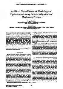
3.5 Optimizing Method Using Genetic Algorithm (GA) In this subsection, we describe the method based on a simple genetic algorithm (See D. Goldberg, 1989 for details). Each individual has a gene whose length is equal to the number of positions at which users can put light sources. The gene that we use is shown in Figure 5. Elements of a gene
1
0
0
2
3
0
4
0
3
1
2
2
Figure 5. Example of a gene. The number recorded in each element of a gene is the light source type number, which is defined in subsection 3.3.1. To get an optimum solution, we continue to refine the genes of the individuals. The cost function we should minimize is
φ1 = A( ∑ (lightk − Rk ) ) 2
k
= A{∑ (lightk ) 2 − 2∑ lightk Rk + ∑ ( Rk ) 2 }, k
where
k
(13)
k
Rk is the obtained illuminance in position k, and lightk is the illuminance value
specified by the user. To minimize this cost function, we use reproduction, crossover, and mutation. In the reproduction stage, good individuals are selected by using roulette rules. The finest individual is always selected; this method is called the elite strategy. In the crossover stage, we select two individuals from a set of comparatively superior individuals, and if they have the same row of genes partly, we combine these two individuals to create a new individual. In the mutation stage, we select individuals at random, and change their gene values at random.
3.6 Optimizing Method Using Simulated Annealing (SA) In this subsection, we describe the method that uses simulated annealing, (See Kirkpatrick et al., 1983, for details). In this method, we repeat to change light sources according to a stochastic rule. If the value of the cost function is decreased by changing a light source , we always adopt the change. However, if the value of the cost function increases, we decide whether to adopt a change of the light source which is turned on or not as follows. The probability is accompanied with the temperature which is defined as follows:
T= where
p , log(t + 2.0)
(14)
p is a constant value and t is a time step. The probability is defined as follows.
P=
1 .0 , ∆energy 1.0 + exp( ) T 10
(15)
where
∆energy is the change in the cost function. The cost function is defined in Eq. (13).
4. Experiments and Results 4.1 Comparison with other methods (neural network, GA and SA) In this section, we compare the performance of the proposed method using the chaotic neural network with other conventional optimization methods. First, we apply these methods to a small size problem which has only 6 positions for placing light sources. The problem is small enough that we can search for the optimum solution using all the states in the searching region. By applying to such a small problem, we can check whether the proposed method or other conventional methods can actually find the optimum solution or not. The behavior of the objective function
φ
of the chaotic neural network is shown in
Figure 6. It is clearly seen that the state of the chaotic neural network does not converge to any state but keeps fluctuating chaotically. This avoids trapping at undesirable local minima and enables an efficient search for the optimum solution. Table 1 summarizes the results of the conventional neural network search with gradient dynamics, the chaotic neural network search, the genetic algorithm search, and the simulated annealing search. These
“Average solution” is the average of the obtained minimum values of the objective
function (the sum of the differences between the illuminance values specified by the user and the obtained illuminance values), over 10 runs. All methods, except for the conventional gradient neural network, can obtain the optimum or nearly optimum solution to the problem.
Figure 6. Behavior of the cost function.
Optimum
Neural
Chaotic
Genetic
Simulated
solution
network
network
algorithm
annealing
11
Average solution
0.0000
0.3983
0.0000
0.0003
0.0000
Table 1. Results for a small problem of 6 light sources.
Next, we show the results for a medium-sized problem in which the number of positions for light sources is 12. For this problem, the globally optimum solution is unknown because we cannot find an exact optimum solution by comparing all states of the searching region in a reasonable time. Table 2 shows the results on the medium size problem. “Average solution” is the average over 10 runs. “Best solution” indicates the best result among 10 runs. “CPU time 1” is the whole CPU time which is consumed by the search. The CPU time for obtaining each optimum result is also shown in the Table 2 as “CPU time 2”. We allotted almost the same “CPU time 1” to all methods. Because the conventional neural network method obviously converged to a local minimum, its “CPU time 1” and “CPU time 2” are equal. Table 2 shows that the proposed method provides the best performance among all methods. The difference between the best solution of the proposed method and that of the simulated annealing method is very slight. However, the average result of the proposed method is obviously superior to the other methods. Neural
Chaotic
Genetic
Simulated
network
network
algorithm
annealing
Average solution
111.6105
11.9918
20.8843
29.2012
Best solution
69.4518
9.6081
10.4602
9.6356
CPU time 1(sec)
0.0129
73.89
81.38
78.52
CPU time 2(sec)
0.0129
46.62
59.65
43.66
Table 2. Results for a medium-sized problem of 12 light sources. Finally, we show the results for a large problem. In this problem, the number of positions in which the user can put a light source is 24. The optimum solution is unknown also for this problem. Table 3 shows the results. The definitions of “Average solution”, “Best solution”, “CPU time 1”, and “CPU time2” are the same as for the medium-sized problem. Our method gives the best
“Average solution” and the best “Best solution”. The larger problem
obviously requires more time, but these results show that our method can find a fairly good solution in a reasonable time.
Neural
Chaotic
Genetic
Simulated
Network
Network
Algorithm
Annealing
Average solution
343.85
111.1873
183.7608
126.2916
Best solution
299.1785
106.1020
134.4682
112.5485
12
CPU time 1(sec)
0.0137
212.8719
236.7853
232.5402
CPU time 2(sec)
0.0137
82.4353
155.5983
140.5285
Table 3. Results for a large problem of 24 light sources.
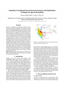
4.2 Results Images
Figure 7. Example of museum lighting design.
Figure 8. Intermediate images.
Figure 9. Example of office room lighting design.
13
Figure 10. Intermediate images. We optimized the lighting in two environments. Figures 7 and 9 show the solutions obtained by the chaotic neural network method. The images are generated by combining the intermediate images in Figures 8 and 10, respectively, each of which corresponds to a firing neuron in the chaotic neural network. Figure 11 shows the ceiling lights seen from the floor. Figure 12 shows the distribution map of the obtained illuminance values. The higher the brightness value of the pixel in the image is, the brighter the place is. Figure 13 shows the specified illuminance values.
Figure 11. Image seen from the floor.
Figure 12. The illuminance distribution map.
14
Figure13. Specified illuminance values.
5. Conclusions In this paper, we have proposed the method based on the chaotic neural network to solve the lighting design problem. We have compared the proposed method with other methods based on the conventional neural network, the genetic algorithm, and the simulated annealing. First, we have shown that our method and other methods except the conventional gradient dynamics neural network have an ability to find an optimum solution of a small size problem. Then, we have applied these methods to larger problems. Compared with other methods, the proposed method using the chaotic neural network has the property that does not require very much time to find a good solution. These experiments imply that as the size of the problem increases, the proposed method shows better performance compared with other methods. It should be noted, however, that the methods with the conventional neural network, the genetic algorithm, and the simulated annealing can be also improved by adding further contrivances. We have examined the obtained images by making an illuminance distribution map and an image which is looked up from the floor. The results show that the chaotic neural network can effectively solve the lighting design problems.
References Aihara, K., Numagiri, T., Matsumoto, G. and Kotani, M. (1986) Structures of attractors in periodically forced neural oscillators. Phys. Lett. A, 116, 313-317. Aihara, K., Tanabe, T. and Toyoda, M. (1990) Chaotic neural networks. Phys. Lett. A, 144, 6, 7, 333-340. Caianiello, E. R. (1961) Outline of a theory of thought-processes and thinking machines. J. Theor. Biol., 2, 204-235. Chen, L. and Aihara, K. (1995) Chaotic Simulated Annealing by a Neural Network Model with Transient Chaos. Neural Networks, 8, 915-930.
15
Cohen, M.F. and Greenberg, D.P. (1985) The Hemi-Cube: A Radiosity Solution for Complex Environments. Computer Graphics, 19, 3, 23-30. Dobashi, Y., Kaneda, K., Nakashima, T., Yamashita, H. and Nishita, T. (1995) A Quick Rendering Method using Basis Functions for Interactive Lighting Design. Computer Graphics Forum 14, 3, C299-C240. Dobashi, Y., Nakatani, H., Kaneda, K. and Yamashita, H. (1998) An Interactive Lighting Design System Integrating Forward and Inverse Approach. The Institute of Image Electronics Engineers of Japan, 27, 4, 394-359. Goldberg, D. (1989) Genetic Algorithms in Search, Optimization and Machine Learning. Addison-Wesley. Hasegawa, M., Ikeguchi, T., Matozaki, T., and Aihara, K. (1995). Solving Combinatorial Optimization Problems using Nonlinear Neural Dynamics. Proc. of International Conference on Neural Networks, 6, 3140-3145. Hasegawa, M., Ikeguchi. T., and Aihara, K. (1997). Combination of Chaotic Neurodynamics with the 2-opt Algorithm to solve Traveling Salesman Problems. Physical Review Letters, 79, 12, 2344-2347. Hasegawa, M., Ikeguchi, T. and Aihara, K. (2000). Exponential and Chaotic Neurodynamical Tabu Searches for Quadratic Assignment Problems. Control and Cybernetics, 29, 3, 773-788. Hasegawa, M., Ikeguchi, T and Aihara, K. (2002). Solving Large Scale Traveling Salesman Problems by Chaotic Neurodynamics. Neural Networks, 15, 2, 271-283. Hopfield, J. J. and Tank, D. W. (1985). Neural Computation of Decisions in Optimization Problems. Biological Cybernetics, 52, 141-152. Immel, D.S., Cohen, M.F. and Greenberg, D.P. (1985) A Radiosity Method for Non-Diffuse Environments. Computer Graphics, 20, 4, 23-30. Kawai, J.K. and Painter, J.S. and Cohen, M.F. (1993) Radioptimization: Goal Based Rendering. Computer Graphics Annual Conference Series, 147-154. Kirkpatrick, S., Galatt, C. and Vecchi, M. (1983) Optimization by Simulated Annealing. Science, 220, 671-680. Nagumo, J., and Sato, S. (1972). On a response characteristic of a mathematical neuron model. Kybernetik, 10, 155-164. Nishita, T. and Nakamae, E. (1985) Continuous Tone Representation of Three-Dimensional Objects Taking Account of Shadows and Interreflection. Computer Graphics, 19, 23-30. Nozawa, H. (1992)
A Neural Network Model as a Globally Coupled Map and Applications
based on Chaos. Chaos, 2, 377-386. Schoeneman, C., Dorsey, J. J., Smits, B., Arvo, J. and Greenberg, D. (1993) Painting with Light. Computer Graphics Annual Conference Series, 143-146. Takahashi, K., Kaneda, K., Yamanaka, T., Yamashita, H., Nakamae, E. and Nishita, T. (1993) Lighting Design in Interreflective Environments Using Hopfield Neural
16
Networks. The illuminating Engineering Institute of Japan, 17, 2, 9-15. Wallace, J.R., Cohen, M.F., and Greenberg, D.P. (1987)
A Two-pass Solution to the
Rendering Equation: A Synthesis of Ray Tracing and Radiosity Methods. Computer Graphics, 21, 4, 311-320. Whitted, T. (1980) An Improved Illumination Model for Shaded Display. Comm. ACM, 23, 6, 343-349. Yamada, T. and Aihara, K. (1997) Nonlinear Neurodynamics and Combinatorial Optimization In Chaotic Neural Networks. Journal of Intelligent & Fuzzy Systems, 5, 1, 53-68.
Appendix 1 Overview of The User Interface Our lighting design system has two phases. The first phase is the preprocessing phase in which we set the viewpoint and illuminance values users desire. The second phase is the optimization phase and by using several programs of Radiance, where Radiance is a collection of free programs about lighting visualization and these programs do many things from object modeling to rendering in consideration of interreflection of lights, image processing, and display, and the optimization program using the chaotic neural network, we render the intermediate images, and extract the illuminance values of each intermediate image and calculate the optimum solution and render the final output image. The flow chart of this system is shown in Figure 14.
2 Preprocessing Program First, we input the 3D object data in which we design interior lighting. Second, we set the viewpoint. To set illuminance values we desire in the next step, we need to make the positions at which we set the illuminance values visible. By changing these x , y and z coordinates, we change the viewpoint and rotate the space. Last, we set the illuminance values users want. We can set the illuminance values at multiple points.
3 Optimization Program First, intermediate images which have only one light source respectively are rendered. Second, the brightness values of pixels where users specified the illuminance values are extracted from all intermediate images. Third, by consulting the illuminance information extracted above, the chaotic neural network searches the optimum solution. The internal states of the neurons are updated asynchronously. The solution which has the smallest quasi energy function is always memorized, and after finite time steps, the solution with the smallest energy is output. Last, according to the best solution, we render the final output image.
17
Loading 3D-geometric model data
Specifying Viewpoint
Specifying Illuminance values
Rendering intermediate images
Extracting illuminance values where a user specified from intermediate images
Optimizing by using the chaotic neural network
Rendering a final image based on the optimum solution calculated the chaotic network Figure 14. The by flow chart of theneural proposed system. Figure 14. The flow chart of the proposed system.
18