Sensor optimization using neural network sensitivity ... - CiteSeerX

Meas. Sci. Techno]. 6 (1995) 1291-1300, Printed in the UK

Sensor optimization using neural network sensitivity measures R Naimimohasses, D M Barnett, D A Green and P R Smith Optical Engineering Group, Department of Electronic and Electrical Engineering, Loughborough University of Technology, Loughborough, LE1 1 3TU, UK Received 21 December 1994, in final form 12 May 1995, accepted for publication 25 May 1995 Abstract. A new method of optimizing a multi-sensor geometry using neural network function fitting and sensitivity measures is described. The method is applied to a multi-angle optical scattering nephelometer for which theoretical scattering intensities are generated for distributions of spherical dielectric particles. Neural networks are trained to invert these angular intensities to determine accurately the size distribution of normally distributed particles. The nephelometer model is optimized to a minimum configuration using the sensitivity analysis. The method is further validated on experimental data by identifying essential channels in an on-line nephelometer used to determine concentration and species of oil-in-water suspensions

1. Introduction

On-line monitoring is used in the process industries to acquire control parameters, to monitor the quality and efficiency of the process and to ensure safety and reliability. Optical sensors are often used on-line [l] for their non-invasive operation, low maintenance requirement and ease of deployment. However, many potentially useful optical systems are not generally installed on-line because of inappropriate technology or a perceived lowcost benefit. Particle size analysis using laser diffraction [Z], for example, is designed for laboratory use when a high resolution measurement is required. Substantial sample preparation and instrument calibration is necessary for all but the most uniform suspensions (e.g. spherical monodispersion). The device most often used to measure particle suspensions on-line is the turbidity 131 sensor whose response, however, is only indirectly and often ambiguously related to the physical properties of the suspension. An advance in this technology would be of interest if it could deliver intermediate resolution information on the physical properties of the suspension, whilst using a sufficiently simple low-cost on-line system. A turbidity sensor can be seen as a low-dimensional limit of a multi-angle scatter sensor or nephelometer [41. A finely resolved nephelometer can deliver useful additional information but the degree of redundancy may be high and therefore its widespread use on-line might be unlikely. This paper describes and extends a technique [SI for the design of scattering sensor systems in which the sensor geometry is optimized for a given information delivery. An artificial neural network [6]is used to model the sensor system and to investigate its sensitivity to particular angular input data. 0957-02331951091291t10$19.50 @ 1995 IOP Publishing Ltd

I

1i

Turbidity= -

IS0

Figure 1. Measure of turbidity. Simulated data are generated using Mie theory [7,8] and these data are inverted to yield accurate information on the physical properties of the particles using only a minimum of input parameters. Real data obtained from an on-line low-resolution nephelometer [9] are also processed using these techniques and it is shown that the system can have a reduced complexity whilst delivering a similar quantity and accuracy of information. Although this technique is applied to the problem of on-line particle characterization, it is a generic method and can equally well be applied to any system whose input vector dimensionality requires minimization. 2. Turbidity and its limitations

Turbidity is ubiquitous as the method for indicating the suspended particle content of a fluid, and is defined as the ratio of light intensities measured across and in the line of sight (LOS) (figure 1). For solutions of sufficiently low particle contamination the LOS intensity is proportional 1291

R Naimimohasses e t al

-.

Figure 2. Turbidity calculated for particles with refractive index relative to background, m = 1.2 and for a range of particle size distributions (normalized to wavelength).

to the source intensity and is virtually independent of the suspension. The turbidity ratio is calibrated against a standard turbid solution (historically formazine) and a linear scale of turbidity is assumed (e.g. nephelometric turbidity unit NTU).In the context of water, for example, turbidity is caused by the presence of suspensions of gas, liquid or solids. In many industries, including the water industry, turbidity is assumed to indicate the mass or volume of suspended particles (in the absence of a more precise measure). The accuracy of this assumption with respect to suspensions of spherical dielectric particles with known size parameters can easily be tested, since an exact scattering solution is available [7]. Scattering simulations from particles having normally distributed sizes were undertaken with the source assumed to be unpolarized and the observation being made in the scattering plane. Particle sizes ( x = ka) are normalized with respect to the wavenumber in the ambient medium (k) and relative refractive indices m = (&pa~c,e/&mbjent) are quoted relative to the refractive index of the ambient medium. Figure 2 shows the calculated turbidity (in arbitrary units) from a series of particles (m = 1.2) normally distributed over a range of mean sizes (&) and standard deviations (U). By holding the number of particles constant the total mass volume varies over the surface like w3 :paz, which follows from the assumed normal distributions. Clearly the turbidity index exhibits significant structure and this is more pronounced as the distributions tend towards monodispersions. A further insight into the behaviour of the turbidity index can be gained by considering particle distributions with constant volume fraction, as shown by the simulations presented in figure 3. Although little detailed structure is observed, except for monodispersions (not shown), a very significant range of output is obtained, indicative of the highly ambiguous interpretations that can be placed on the turbidity measure. The variation of turbidity with particle refractive index (m)is summarized in figure 4, using data derived from simulations similar to those performed in

+

1292

Figure 3. Turbidity as a function of particle size distribution for constant volume fraction and for refractive index relative to background (a) m = 0.8,(b) m = 1.2 and (c) m = 50.

Sensor optimization using neural network sensitivity measures

J

I

0.01 0.8

1

1.2

1.4

1.8

1.6

2

Refractlve index (relative to background Index) Figure 4. Turbidity as a function of particle refractive index (m) over a range of particle size distributions with constant volume fraction. Forward scattered light intensity

''S

I

Standard deviation

20

-0-0.85

15

-1.1

IO

5 25

30

35

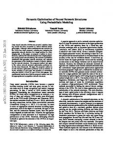
Mean particle size Figure 5. Forward scattered light intensity versus mean particle Size over a range of standard deviations. (For air bubbles in water, m = 0.75.) the compilation of figure 3. Once again it is apparent that turbidity is not uniquely indicative of any physical property of the particle distributions. Nevertheless turbidity is clearly afinction of the particle type and size distribution and as such contains information about these properties. It is interesting to speculate on what further degree and type of information would be required to resolve the ambiguity and so to enable the design of an efficient sensor. It is well known that accurate particle sizing can be performed using instrumentation measuring more distributed scattering than the turbidity [IO]. For instance, the mean particle size can be readily extracted from the forward scattered light intensity, having little dependence on the standard deviation of the particle size (figure 5). For large particles a simple diffraction model is sufficient to associate scattering angle with size and for smaller (order wavelength) size particles the Mie theory can be used to fit the data provided the optical property of the

particles is known and the particle shape does not depart significantly from spherical. When these conditions are not satisfied, representative results may still be obtained since averaging effects can reduce the significance of shape and composition. Instrumentation used to perform these measurements are large scale, laboratory based systems unsuited for on-line deployment where a simple solution yielding mean and variance of the size distribution would be a major advance. However, extracting size variance information on-line is not such a trivial problem as there is insufficient relevant information available from any one sensor. This reflects the fact that standard deviation exhibits a complex relationship with the observed intensity and the mean particle size (figure 2). The complexity of this dependence is such that it is very difficult to approximate a solution using conventional multi-dimensional curve fitting techniques. 1293

R Naimimohasses et a/

(a) Estimated mean 36 1

26

25

27

28

31 32 Actual mean particle size 30

29

33

35

34

Estimated stanadard devlatlon 1.6 1.61.41.2 --

1I--

O A -. 0.8

t

1

0.6 -.

A

0.4 -0.2

-.

4,&

,

O/ 0

0.2

0.8 1 1.2 AEtUal standard deviation in particle size 0.4

0.6

1.4

Figure 6. ( a ) Estimated mean particle size versus &he actual mean (for various standard deviations), approximated by ANN having three input angles go', 175' and 180" from launch. (b)Estimated particle size standard deviation versus the actual deviation, for a range of mean sizes (25-35), approximated by ANN having five input angles go", 120", 135", 175" and 180" from launch. (c) Estimated particle size standard deviation versus the actual deviation, over a range of means (25-35). The ANN incorporates an additional input (estimated mean particle size) with the angular inputs used in obtaining (b).

3. Sensor modelling using artificial neural networks Artificial neural networks (ANNs) are nonlinear data processing systems whose behaviour is analogous to the workings of the human brain. They learn by example, that i s an untrained network i s presented repeatedly with examples of the function they are to learn. One such 1294

architecture, the multi-layer perceptron (MLP) starts in a random empty state and propagates the training information through the network using a back-propagation [ l l ] error gradient decent algorithm. I t has been shown [I21 that a sufficienlly large MLP can be used to model any nonlinear function to arbitrary accuracy [13-15]. Given the complexity and nonlinear nature of the intensity profiles of the scattered light intensity, i t i s an ideal exercise for an

Sensor optimization

().

using neural network sensitivity measures

Estimated standard deviation 1.6

0.0

0.2

0.4

0.8

0.6

1.O

1.2

1.4

Actual standard deviation in particle size Figure 6. (Continued) A" to model. A training set for the ANN was produced using exact Mie theory 161. Each input-output training pair in the set consists of integrated intensities at various scattering angles versus the desired mean or standard deviation. The theoretically calculated intensities, having a size distribution given by n(orj. are given by a Fredholm integral of the first kind as

~ ( e=)

im

I(~,LY)~(u)~cY

inputs

hidden

outputs

layer

(1)

where c( is the particle size and it is further assumed a constant index ratio m = 3/4 (air bubbles in water). These data were presented to two different networks, with the angular intensities forming the input vector and the particle size parameters used as the output vectors. The ANN was thus trained to l e a the inverse of the Mie problem in determining the statistical parameters (mean and standard deviation). There is a nonlinear relationship between I ( 0 j and the particle distribution parameters (@,U) [17]. A good fit to the mean was achieved and an acceptable fit to the standard deviation (see figure 6). The mean can be estimated using just three angles whilst retaining an accuracy of 99.8%. Five angles were needed to estimate the standard deviation, giving an accuracy of 90.6%. It is well known that inverse solutions of the Fredholm equation ( l j are ill-posed in the sense that the inversion is nonunique and unstable to the presence of noise in the input data set. In seeking regularized inverse solutions authors have incorporated statistical constraints [NI, including least mean square, and or a priori 'knowledge such as data bounds [ 191. Since ANNs are data mapping functions whose leaming methods are based on statistical criteria, they have inherent regularization properties and for that

Figure 7. A two-layer MLP with d inputs, m sigmoidal hidden units and a linear output node. The weights connecting the input layer to the hidden layer are labelied by subscript vi) and those connecting the hidden layer to the output by (lj).Outputs from the hidden layer are indicated by q. reason are often applied where noise is a particular problem [20]. In the example considered here, the nonuniqueness of the inverse solution is reflected in the determination of standard deviation, exhibiting departures from the desired values (figure 6(bjj. It is clear that further domain knowledge is required to regularize the inversion which could for example take the form of a priori knowledge of the mean particle size. Figure 6(cj shows the effect of incorporating this extra input to the inverse mapping obtaining an overall accuracy of 96% for 1295


Epoch

1500 2250

3000 3750

Sensitivity 7

I

7 5

LLJ"

Epoch

3000

3750

Figure 8. Training and minimization of neural network model (to exact Mie theoretical results): (a) mean-square error during training of mean, (b)input sensitivity during training of mean, (c) mean-square error during training of standard deviation, (d) sensitivity during training of standard deviation. the inversion results. The main purpose of this paper is to describe a method for sensor design based on a functional representation (i.e. ANN) of a data mapping. We are not primarily concerned with inverse scattering solutions since they depend on the existence of a forward scattering solution and not simply on observations of the scattering The above example has been included phenomena. to demonstrate the capability of ANNs in performing regularized inverse mappings on a canonical problem. We now return to the practical applications of sensor design and data mapping.

involve lengthy data fitting processes in conjunction with extensive statistical analysis [21,22]. In this neural sensor design approach, the techniques of information content analysis and data fitting are integrated into a single neural network based design methodology. An MLP learns to perform a smooth input-output functional representation from observations and hence it can be considered as a method for intelligent function prototyping. A sensitivity matrix can be calculated for input (z) and output (y) vector arrays over the training patterns 4 given by,

4. Sensor design

Optimal sensor design is the process by which a maximum amount of information is extracted whilst the number of sensors is minimized. Conventional techniques for determining information content of any single sensor 1296

Considering an MLP with squashing function (e.g. sigmoid), chis calculation is readily incorporated into the backprop training algorithm with minimum overhead. For a conventional two-layer MLP performing a function


Figure 8. (Continued)

estimation as depicted in figure 7, having sigmoidal activation function for the hidden layer elements and a single linear output node, the differential sensitivity t e m s can be determined by the chain rule as s;l,

c

c m

~ Y I ~ Y Im azj = -= - = w1.j axi azj j = l axi j=l

WjiZj(l

- Zj). (3)

The overall computational overhead involved in the sensitivity calculation is of the order of O(m x n ) operations for the n learning patterns and m hidden nodes which need only be evaluated once after the training is completed. It has to be noted that S is a general measure and works with most learning algorithms provided that the network response is continuous. Boolean and digital type outputs due to the discrete nature may need some modification due to the zero valued differential over the quantization level. The total sensitivity is determined by calculating the statistical significance of the contribution due to each individual sensor (i.e. input) over all training patterns. The average of the sensitivity modulus over the training set is used as this measure. The mean sensitivity can then

he plotted as a function of training epochs giving trends of relative input sensitivity. The heuristic optimization methodology used for minimizing input parameters can be summarized as: (i) start with a sensible network size, (ii) train the network to a minimum error, (iii) calculate sensitivity matrix, (iv) remove the least sensitive input by nulling the associated weights, (v) go to step (ii). This procedure is repeated until subsequent deletions cause a substantial decrease in the network performance (i.e. significant permanent increase of mean-squared error (MSE)). The optimal network configuration may be found by repeating the same procedure applied to different initialized networks combined with network pruning techniques for improved generalization [23-251. The results from an example of such a training and input deletion process can be seen in figure 8. The networks were originally trained for 750 epochs (that is 750 presentations of each of the training patterns available) before any input 1297


Figure 9. Training and minimization of neural network model (to experimental nephelometer data): ( a ) mean-square error during training of type detection, ( b ) sensor sensitivity during training of type detection, (c) mean-square error during training of concentration, ( d ) sensor and type sensitivity during training of concentration.

deletion has taken place and each further input deletion is similarly preceded by 750 epochs. The decay in error can be seen in figures 8(a) and 8(c), from which it can be deduced that only a small increase in error occurs when an input with little or repeated information is removed from the network. Figures 8 ( b ) and 8(d) show the increasing sensitivity of each input across the training process, with input sensitivity going to zero when the input is deleted. It can he clearly seen how only a few of the inputs contain the majority of the information required for the functional predictions (50%reduction in input dimensionality and 45% reduction in network size). 5. Experiment

To test these ideas in practice, data from an on-line nephelometer [9] were obtained, using suspensions of oil-in-water. The experimental system consisted of a nephelometer measuring six azimuthal angles of 45", 90", 135", 180", 240" and 300" measured from the launch (i.e. 0"). The experimental data were gathered covering the concentration range of (0-100) parts per million (PPM). Three oils were used in this study, namely motorcycle 1298

fork oil, Hams crude oil and soluble oil, each exhibiting different scattering characteristics. For each oil species and concentration (at intervals of 10 PPM), five independent measurements were taken giving a total data sample of 165. For each data set, the background water and oil suspensions were different and the experiments were conducted by different people on different days and under different environmental conditions. These data were subsequently normalized [9] to compensate for drifts in electronics as well as source variations. Four sets of gathered data, picked at random, were used for training the network, while the remaining data set was used to measure the network performance (i.e. testing data). The artificial neural network structure used was a concatenated feed forward MLP [9]. This structure utilizes the maximum information embedded in the mediums scattering signature by a task division multiplexing scheme. At first, a MLP was trained to recognize the oil type, ope network, and subsequently this decision was used as a coded input for the concentration network to be used as an a priori knowledge of particle type. Figures 9 ( a ) and 9(b) respectively show the percentage error (% error) and the sensor sensitivities as a function of


Figure 9. (Continued) the training epochs for the type detection task. The initial network has S inputs, 7 hidden layer nodes and a linear output with a tri-state coding of the types (soluble oil= 1, Hams crude oil= 2 and fork oil= 3). The network was initially trained to SO00 epochs before each input deletion. As is seen from figure 9(a), % error remains reasonably low for up to 2 sensor deletions. The two sensors deleted were the 45" and 90" sensors as is seen from figure 9(b). The third sensor deletion resulted in a classification failure. The result also shows how the individual sensor sensitivities reorder their ranking following a deletion, reflecting the way in which the network attempts to equalize the flow of information from input to output vectors. Also note that the 90" sensor is only slightly less sensitive than the 300" S e n S ~ rwhich then aSSumeS significantly increased sensitivity when the former is deleted (at 10000 epochs), implying that these sensors contain much of the same information concerning type identification. The output of the type network is used as an additional input to the concentration network, which has 6 inputs, IS hidden layer nodes and a single sigmoidal output node. The concentration is normalized to a zero to one range for the dynamic range of the sigmoid. This network configuration produced the optimum learning. Figure 9 ( c )

shows the % error of the network for both training and testing data sets. The concentration network was trained for 10000 epochs between sensor deletions. This figure clearly indicates that network performance is not degraded by deletion of four sensors (4S", 90", 240" and 300"). Figure 9(d) shows the sequential deletion pattern as the network is being trained. The concentration is successfully obtained from only the 135" and 180" sensors together with the type input. It is interesting to note that following the deletion of the 300" sensor, the type input becomes very important for successful prediction, reaffirming the role of that particular sensor in oil type detection, viz figure 9(b). It may be concluded that the nephelometer with minimized design complexity for the combined task of oil type classification and concentration estimation in the range 0-100 PPM will have the following Sensor geometry (135", 240", 300" and 180"). 6. ~

~

~

~

l

This paper has outlined a technique for the design of improved on-line sensors for particle sizing and characterization. A theoretical model was used to explore the limitations of existing technology and to produce 1299

R Naimimohasses et a1

synthetic data to test the design methodology. The initial sensor designs respond to light scattered at a range of angles, although it is not obvious how useful this additional information is. Tnis problem was addressed by the development of a sensitivity analysis which uses artificial neural networks to optimize and minimize the complexity of the sensor geometry. The methods described in this paper are similar to those in the wet1 documented area of network pruning [23-271. Whereas, network pruning works towards minimizing the network complexity by deleting connections and hidden units, this method deletes inputs, thus minimizing input dimensionality. Pruning methods are of interest in neural network studies, this method is of more interest to those in sensor design. The method was successfully used in training an ANN to model a multi-input sensor and then to minimize the sensor's input dimensionality. The number of inputs presented to the network, and hence the sensor complexity, can be reduced systematically whilst keeping the error within reasonable and acceptable bounds. Validation of the design method was demonsmated by application to on-line sensing of oil-in-water suspensions. A nephelometer with reduced complexity was designed to deliver the type and concentration of oil in the range 0-100 parts per million by volume. The methods used are not in any way application specific and although our own interest is focused on sensing in the process industry, the technique is applicable to any design, minimization or optimization problem in wh'kh a data model is appropriate. The analysis of turbidity performed here will have implications in future, improved measures of suspended particle content not least because the optimization process is driven by data rather than theory and is therefore applicable to real on-line systems. Extensions of the basic principle which are of relevance to the process control industries include constrained optimization, selfoptimization nnd performance monitoring.

Acknowledgment

DAG is supported by an EPSRC grant number GR/H45261. References

--

111 - - Briees R and Grattan K T V 1990 The measurement and sensing of water quality: a review Trans. Inst. Meas, Cont. 12 65-84 (21 Hunter R J 1993 Introduction to Modern Colloidal Sciences (Oxford: Oxford University Press) pp 57-96 131 Clesceri L S, Greenberg A E and Rhodes Trussell R 1989 Standard Methods for the Examination of Water and Waste Water 17th edn American Public Health

Association, Washington, DC 141 McCartney E J 1976 Optics of the Atmosphere ch 5 (New York Wiley) [SI Naimimohasses R, Bamett D M, Green D A and Smith P R 1994, An approach to opto-neural sensor design for

1300

process monitoring IOP Conf. on Applied Optics and Optoelectronics. (York. UKJ 5-8 September pp 349-51 [61 Bishop C M 1994 Neural networks and their applications Rev. Sci. Instnun 65 1803-32 (71 Mie G 1908 Beitrage zur optik truber median, speziell kolloidaier metallosingen Ann. Phys. 25 377-445 [SI van de liulst H C 1957 Light Scattering by Small Particles (New York: Wiley)

191 Smith P R, Green D A and Naimimohasses R 1994 Some investigations on neural processing of scattered light in water quality assessment I E E Proc. Ws.Image Signal Process.

[IO] Coston S D and George N 1991 Recovery of particle size distributions by inversion of optical transform intensity Opt. Lett. 16 1918-20 [ I 11 Rumelhart D E, Hinton G E and Williams R J 1986 Learning internal representations by error propagation Parallel Distributed Processing: Explorations in the Micmstructure of Cognition vol 1 (Cambridge, MA:

MIT Press)

W 1986 Neural networks for computation: number representations and programming complexity Appl. OpL 25 3033-46 [131 Cybenko G 1989 Approximation by superposition of a sigmoidal function Math. Cont. Signals Syst. 2 303-14 E141 Kolmogorov A N 1957 On the representation of continuous functions of many variables by superposition of continuous functions of one variable and addition Dok Akad. Nauk. 144 670-81 [IS] Hornik K 1991 Approximation capabilities of multilayer feedforward networks Neural Net. 4 251-7 [I61 Zijp J R and Tenbosch J J 1993 Pascal program to perform Mie calculations Opt. Eng. 32 1691-5 1171 Ishimaru A, Marks U R J. Tsang L, Lam C M, Park D C and Kitamura S 1990 Panicle-size distribution determination usinE ootical sensine and neural networks Opt. Lett. 15 122113 . U81 nkhonov A 1963 Solution of incorrectlv formulated problems and the regularisation methbd Sov. Math. Dokl. 4 1035-8 1191 Miller K 1970 Least squares methods for ill-posed problems with a prescribed bound SIAM J. Math. Anal. 1 52-74 [201 Kulkarni A D 1991 Solving ill-posed problems with artificial neural'networks Neural Net. 4 477-84 [U]Miller J C and Miller J N 1993 Statistics forilnalyrical Chemisfry 3rd edn (Englewood Cliffs, NJ: Prentice-Hall) 1221 Graham R C 1993 Data Analysis for the Chemical Sciences, A Guide to Statistical Techniques (Heidelburg: VCH) [23] le Cun Y, Denker 1 S, Henderson D, Howard R E , Hubbard W and Jackel L D 1990 Optimal brain damage Advances in Neurai Infor,nation Pmcessing Systems vol 2, ed D Touretzky (San Mateo, C A Morgan Kaufmann ) [24] Hassibi B and Stork D G 1993 Second order derivatives for network pruning: Optimal brain surgeon Advances in Neural Information Processing Systems vol 5, ed S J Hanson (Morgan Kaufmann) 1251 Nowlan S 1 and Hinton G E 1992 Simplifying neural networks by soft weight sharing Neural Comput. 4 473-3 1261 Karayiannis N B and Venetsanopouios A N 1993 Artijkial [121 Takeda hl and Goodman J

I

Neural Networks, Learning Algorithms, Performance Evaluation and Applications (Deventer: Kluwer)

1271 Lapedes A and Farber R 1988 How neural networks work Neural Information Pmcessing Systems ed D Z Anderson (New York: American Institute of Physics) pp 442-56