Optimized 3D ray tracing algorithm for environmental acoustic studies Matthieu DREHER, Guillaume Dutilleux, Fabrice Junker
To cite this version: Matthieu DREHER, Guillaume Dutilleux, Fabrice Junker. Optimized 3D ray tracing algorithm for environmental acoustic studies. Soci´et´e Fran¸caise d’Acoustique. Acoustics 2012, Apr 2012, Nantes, France. 2012.
HAL Id: hal-00811045 https://hal.archives-ouvertes.fr/hal-00811045 Submitted on 23 Apr 2012
HAL is a multi-disciplinary open access archive for the deposit and dissemination of scientific research documents, whether they are published or not. The documents may come from teaching and research institutions in France or abroad, or from public or private research centers.
L’archive ouverte pluridisciplinaire HAL, est destin´ee au d´epˆot et `a la diffusion de documents scientifiques de niveau recherche, publi´es ou non, ´emanant des ´etablissements d’enseignement et de recherche fran¸cais ou ´etrangers, des laboratoires publics ou priv´es.
Proceedings of the Acoustics 2012 Nantes Conference
23-27 April 2012, Nantes, France
Optimized 3D ray tracing algorithm for environmental acoustic studies M. Drehera, G. Dutilleuxb and F. Junkerc a
INRIA Rhˆone-Alpes, ZIRST 655 Avenue de l’Europe Montbonnot 38334 Saint Ismier cedex b Laboratoire R´egional de Strasbourg, 11, rue Jean Mentelin, 67035 Strasbourg Cedex 2, France c EDF R&D, 1 Avenue du G´en´eral de Gaulle, 92141 Clamart Cedex, France
[email protected]
1537
23-27 April 2012, Nantes, France
Proceedings of the Acoustics 2012 Nantes Conference
Ray tracing is a well known algorithm for the generation of realistic synthesis images. It is also applied in the acoustic domain. The computational cost of the full 3D algorithm was previously an obstacle leading to approximations like the 2.5D ray tracing. Despite the fact that this method significantly reduces the needed computations, it also limits the realism of the approach. This article proposes a study of the 3D ray tracing algorithm in the environmental noise context. It presents several methods which can be used to reduce the computation time using different acceleration structures. Design decisions and optimisations made on the general ray tracing engine are explained. Then the choice of the acceleration structure and the propagation method to use is described. The implantation is tested in Code TYMPAN provided by EDF R&D using the NMPB08 method. To conclude, different results are discussed.
1
Introduction
divided into two steps: the geometric step and the acoustic step. The aim of the geometric step is to find the relevant propagation paths between S and R which may include reflections and diffractions on all the obstacles. In the current softwares this step is based either on the ray tracing approach introduced in room acoustics by Krokstad et al. [15] or on the image-source method [4]. This paper deals mainly with the geometrical step. In the past, a 3D computation was not feasible on the hardware available to noise consultants, either because of a too large computational time, or because of excessive memory requirements. Contrarily to room acoustics, due to the overall geometry of the problems addressed where one dimension is much smaller than the two others, and due to the comparatively very large number of objects to take into account in outdoor sound propagation, the search for geometrical paths implemented in the current commercial softwares is carried out in 2.5D. 2.5D means that propagation path are identified first on a horizontal projection of the site. Once horizontal propagation paths have been found, each of them is processed separately in a vertical plane. If interactions with obstacles (reflection(s) and/or diffraction(s) occur along a path, each interaction creates a new vertical plane. In the general case, the set of vertical planes between a source and a receiver is unfolded like a Chinese screen. The second step is to compute the acoustic attenuation between source and receiver in the unfolded vertical plane. This task can be carried out by different methods and standards like ISO9613-2[13], NMPB2008[5], Harmonoise[20], Nord2000[18]. NMPB2008 is the official French method. It is now published as a standard [3] and applies to road, rail and industrial noise. It is beyond the scope of this paper to describe its principles. The reader shall refer to [5] for more details on this method. One essential geometrical aspect of this method which is shared with ISO9613-2 [13] is that reflections on the ground a taken into account by a ”ground effect formula”. It must be emphasized that the distinction between geometric and acoustics issues is not completely clear-cut, since acoustic considerations are certainly of interest for instance in the discretization of the ground or of the obstacles for instance in the selection of ”relevant” propagation paths.
Finding sound propagation paths between sources and receivers can be achieved by using several methods such as image-source algorithm, beam or ray tracing. Major challenges for all these techniques are the accuracy and the computational efficiency. When traversing a scene, a large set of paths have to be considered from source to receiver which can be costly. In the context of outdoor sound propagation, this problem has led historically to simplifications such as the 2.5D ray tracing method. 2.5D is still the standard approach in commercial software. A successful 3D ray-tracing method has to address efficiently three different issues: the geometric complexity of the scene, the representation of the acoustic phenomena, and how to propagate the paths efficiently. In this paper, we propose a study of a 3D ray tracing algorithm applied to environmental acoustics. We describe the different methods we used to solve the three problems listed above and discuss the strengths and weaknesses of our solutions. One of our major preoccupation is the genericity of the proposed ray tracing method. In other words, the ray tracing has to be relatively independent of the acoustic method. Here, we will use the Nouvelle Methode de Prevision du Bruit 2008 (NMPB08) [5] as an application of our method. This paper is organized as follows. Section 2 reviews previous work in geometric acoustic modeling for environmental studies. Section 3 provides an overview of our ray tracing method, the different structures we use and how this ray tracing method is combined with the NMPB08. Section 4 presents experimental results and discusses about the current state of the method and its shortcomings.
2 2.1
Related Work Current practice in environmental noise
In the context of environmental noise impact studies of road, rail or industrial infrastructures and large scale noise mapping in the framework of the European Noise Directive (END)[7], geometric acoustics is currently the most commonly used approach because it appears to be the best tradeoff between uncertainty on the predicted levels and computational burden. Moreover it is quite capable to handle arbitrary configurations of ground profile, reflecting and diffracting obstacles like buildings or noise barriers. Since the physical noise sources are systematically discretized into point sources, the noise impact of a given project can be assessed if one is able to compute the noise level generated at a receiver R by a source S. In the framework of geometric acoustics, the computation between S and R is usually
2.2
Geometric propagations methods
One of the main challenges in the acoustic ray tracing is to find all the possible paths between a source and a receiver, or at least the main ones. Classical ray tracing is very sensitive to the sampling of rays and some paths could be missed if the number of rays is not sufficient. To guide the propagation of the rays, several methods have been proposed. In order to improve the pertinence of the rays, one of the first optimiza-
1538
Proceedings of the Acoustics 2012 Nantes Conference
23-27 April 2012, Nantes, France
tions was to implement ray-tracing from the receiver, which proves to be more efficient in the case of a linear infrastructure. More recently, others have introduced visibility tests of obstacles from a source, a point of interaction or a receiver [17, 8]. Another important method is the beam tracing [10]. The main idea, which is followed in [6] too, is to precompute a tree of visibility between the shapes, the source and the receiver. To do so, beams or frustums are generally used as a superset of all the possibles rays. The main advantage of this method is that the construction of the tree is not subject to sampling and ensures to find all the potential sequences of shapes from sources to receivers. The image-source method [4] is one of the most common to find the reflected paths. However, the complexity of this algorithm is in O(N r ) where N is the number of faces in the scene and r the desired order of reflexion. An extension to this model have been proposed to handle the edge diffraction using the same method [6].
2.3
a face is cut by the plane, its reference is duplicated on both sides. As for the BVH, the choice of the plane is very important and can be computed using the SAH heuristic. For a long time, this structure has been regarded as the best one. However, both BVH and Kd-tree currently achieve comparable performances depending of the type of the scene. A comparison between of the different methods to subdivide a scene is proposed in Figure 1.
3
An efficient 3D ray tracer
Our ray tracing method is made of 2 phases. A precomputation phase selects the areas where the rays should go (according to a particular acoustic method) and builds an efficient data structure called acceleration structure in the following. During the propagation phase, the rays are casted in direction of the relevant areas selected before. This way, we are sure that all the rays casted during this phase could be relevant. In this section, we will focus on three key aspects of our ray tracing method: how to choose an acceleration structure, how to model an acoustic method and finally how to build and use the targeting system. The rest of this ray tracing method consist of the usual ray tracing which is widely described in the literature.
Acceleration structures
Details of the presented structures are beyond the scope of this paper. A full description of these structures and implementation details can be found in [16]. The primary computation cost in the ray tracing algorithm is the ray-scene intersection which complexity is in O(N) with N the number of faces in the scene. The acceleration structures efficiently reduce this complexity to O(log N). These structures have been studied for more than two decades especially in the computer graphics. A survey can be found in [21]. Briefly, we can define three main structures: the Uniform Grid, the Bounding Volume Hierarchy and the Kd-tree. The Uniform Grid [9] is one of the simplest acceleration structure. It uses a regular spatial subdivision of the scene to create cells. When a ray traverses the grid, the ray intersects the faces contained only in the current cell. The main advantage of this structure is its simplicity and rapidity to build. Its drawback is its lack of adaptation to the scene. It is possible that some cells contain no face while other can contain hundreds of faces which can lead to a significant drop in performance. This structure is more suitable for uniformly distributed faces. The Bounding Volume Hierarchy (BVH) is an object-based subdivision [11]. It creates a tree based on the bounding box of the faces present in the scene. The set of faces is recursively divided into two subsets. Unlike the uniform grid, the structure has to choose how to subdivide the set of faces. This criterion is the key point of the performance of the structure. A simple way to subdivide the set is to divide the set in two equally sized subsets but it might lead to low performances. A commonly used heuristic to choose how to divide a set is the Surface Area Heuristic (SAH). Based on the sizes and repartion of a set of faces, this heuristic gives the theoretical best split. This criterion helps also decide to continue the recursion or not. Using the SAH, the BVH is a commonly used structure in the computer graphics domain. It performs very well on a large set of scenes. The Kd-tree [12] is a space-based subdivision. For each subdivision, a plane is chosen to cut the current set of shapes in two parts. The faces related to the current node are then separated from one part to another of the selected plane. If
3.1
Choice of the acceleration structure
As described in the previous section, all the three structures have their own strengths and weaknesses. For each scene there is one more suitable structure to chose. Since the primary goal of this ray tracing method is to be as generic as possible regarding the acoustic method, we cannot make any assumption on the configuration of the scene. The only important feature of the BVH and Kd-tree that we use is the SAH heuristic as it should improve the performances for most of the scenes. In general, the main goal of the acoustic scenes is not to be photorealistic but to represent roughly the objects which are essential to sound propagation. Theses approximations lead generally to scenes with bigger faces comparatively to graphic scenes. For space-based structures (Kd-tree and Uniform Grid), this means that there is good chance that lots of faces are replicated in the different nodes. For objectbased structure (BVH), we can expect relatively big nodes even near to the leaf of the tree. To deal with these problems, two solutions can be: mail-boxing for the spatial based structure and spatial BVH for the object-based structure. The mail-boxing is a technique which prevents a ray to intersect multiple times the same face, saving computation time. The spatial BVH [19] was proposed to deal with large architectural models in computer graphics. It allows the BVH to create nodes by using a plane in the same way as the Kd-tree does. This feature showed a significant improvement in the performance for these scenes. As there is no perfect structure which will outperform the others in all scenes, we feel like it would be too strong a limitation to use only one structure. So, we choose to let the three structure available for the user in our ray tracing method. The implementation of these structures is based on the PBRT system [16]. The benchmark of these structures on different scenes is presented and discussed in section 4.
1539
23-27 April 2012, Nantes, France
Proceedings of the Acoustics 2012 Nantes Conference
(a) Uniform Grid
(b) BVH
(c) Kd-tree
Figure 1: Example of a scene subdivide by a Uniform Grid, BVH and a Kd-tree. In a Uniform Grid1(a), all the nodes are on the same level. For 1(b) and 1(c), the red node correspond to the root level of the hierarchy, the green nodes correspond to the level 1 and the blue nodes correspond to the level 2.
3.2
Interaction with the acoustic model
S
The main interaction between the geometric ray tracer and the acoustic model is in the generation of the secondary rays. When a ray hits a surface, the acoustic method has to describe the ray behavior. To do so, we provide a simple interface to the programmer who has to describe two independent but complementary functionalities: how to generate secondary rays for the first one and answers if an arbitrary ray could have been generated by the current event. Generating the responses is the functionality which computes all the possible secondary rays in the current acoustic event (or at least some samples). For instance, for the specular reflexion, this functionality produces only one ray which is the reflected ray. For the diffraction, it generates a set of rays on the surface of the Keller’s cone of diffraction [14]. The second functionality makes the opposite job. Given a point in space, it answers if this point is reachable by the current event. This feature will be very important in the next section. The acoustic model may also interact during the main loop of the ray tracing algorithm so we have to let entry points at different stages in the loop. For now, we identified four different entry points. The first one is after the scene has been loaded: some informations such as the detection of diffraction edges could be added to the scene for the acoustic model and do some precomputations. The second entry point is during the traversal through the acceleration structure. Usually, these structures are used to find only the first intersection between the current ray and the scene. For acoustics, this could be a limitation so we allow the programmer to choose between different behaviors during the traversal step such as to keep only the first intersection or everything before the first blocking intersection. Figure 2 shows an example of these different behaviors. The third is when a intersection is validated and an acoustic event has to take place. The programmer can choose, given the intersected face and its material, how the ray should continue. The programmer can also choose to terminate the ray because of energy consideration or a too high order of reflection. The fourth is when a complete path is found from source to receiver. The programmer can apply different treatments like filtering or checking.
D1
D2
Figure 2: The diffraction edges(D1,D2) create a volume around the edge which is non blocking. When a ray intersects only the first face, the path which can be found is S-R (green) and S-D1-D2-R (blue). When all intersections before a blocking face are allowed, the four diffracted paths are found. This strategy is used with NMPB08. ery acoustic events, some paths can be overlooked. Moreover, the probability to find a path at a given sampling drops with the distance which is a big problem especially for environmental scenes. The image-source method proposes a solution to eliminate this problem but the computational cost is high and it only works for specular reflexion. We propose a solution based on a targeting system. For a given acoustic method, we assume that we know the relevant area where the acoustic event should occur. For example, receivers are obviously interesting locations for the rays to go. Other interesting areas are the edges producing diffractions. The idea is to sample these areas with a certain density of points (except receivers which are sampled with only one position). The points generated by this sample step are called targets. The generation of these points can take place after all the scene has been loaded and other volumes have been generated (edges for example). In the propagation phase, when a ray hits a surface and an acoustic event occurs, we would like that the secondary ray goes in priority in direction of the targets. To do so, when a event occurs, the system requests all the targets located around the acoustic event and for each target we check if the ray can reach it. With this system, we can guide the rays to any relevant area and solve the problem of distance. An example of this method is presented in the Section 3.4.
3.4 3.3
R
Guiding the propagation of the path
The ray tracing is a very robust and simple algorithm but one of its main weaknesses is the sensitivity to sampling. If not enough rays are generated from the sources and after ev-
Application of the ray tracing method for NMPB08
NMPB08 describes two phenomena: specular reflection and diffraction. We implemented the event interface for both following the Snell-Descartes law of reflection and the Ge-
1540
Proceedings of the Acoustics 2012 Nantes Conference
23-27 April 2012, Nantes, France
ometrical Theory of Diffraction [14]. To detect the edge of diffraction we use oriented bounding boxes (to give a thickness to the edge) which are generated during the post-processing of the scene (entry point 1). During the loop phase, we have to validate reflection and diffraction considering a maximal order and nature of the material encountered. The diffractions are only validated on the augmented volumes that we defined in the post-processing stage. The reflexions are only validated with vertical non natural polygons as NMPB08 includes ground reflexions in the direct path. In other words, rays with reflection on the ground are of no interest in NMPB08. In addition, the length of a path can not exceed 2000 meters in NMPB08. If one of these criteria is not met, the ray is discarded and the loop proceeds with a fresh ray. The diffraction edges and vertical non natural polygons are identified as areas of interest, so they are sampled in the post-processing stage. As the ray tracing algorithm can produce several times the same path, we filter the path found to only validate the shortest ray for a given path. In order to use targeting, we have to introduce a few deviations in the paths. In the case of diffractions, we would like to allow rays to be generated not only on the surface of the diffraction cone but slightly up or under with a given tolerance angle α. For the specular reflection, we check the difference angle between the exact reflected ray and the ray in direction to the target. All along the propagation of the ray, we keep a track of the error made on each event and if the error becomes too important, we simply discard the ray.
4
Results and discussions
4.1
Acceleration structures
To experiment our structures, we generate a very large set of rays and test the intersection with the scene for the 3 different structures introduced in Section 2.3. As the acceleration structure is known to be ”view-dependent” we generate our rays totally randomly. This scenario is considered the worst case one because it removes all convergence in the rays which can lead to a drop of performances. This decision is made because of the divergence of the rays in acoustic modelling which is highly increased by the order of diffractions. For these experiments, we use scenes which are suitable for NMPB08. They are generally composed of a large topography and a few buildings. As an experimental environment, we use the Code Tympan [1] providing by EDF R&D to load and visualize the scene and results. The results in Table-1 are presented using a Intel i7 Q720 @1,6GHz on only one core.
Shapes 121 1080 30924
Kd-tree 304 75 153
BVH 356 61 83
4.2
Propagation of the path
To help finding the relevant paths, the main obstacle is the sensitivity to sampling. We proposed in the section 3 a first approach to guide the rays to interesting places. Table 2: Comparison between random ray tracer and guided ray tracer. The sources contain 10000 rays and 2 diffractions (200 rays per diffraction) are allowed. The target system is enabled for primary rays and first order of diffraction. Scene Simple scene
Shapes 121
Samples 10040
Random 225
Guided 13246
The Table-2 shows the number of paths found by the random ray tracer and the guided ray tracer. As we can see, there is a significant improvement for both scenes with the same parameters in the scene (same number of rays per source and per diffraction). Yet, the computational cost for this framework is still high because of the complexity introduced by the number of samples. When an event occurs, the ray tracer requests all samples around the event which takes time. Then, when all the targets are found, it still needs to check if the targets are geometrically accessible. These operations can be time consuming. For now, the system couldn’t handle scene with several ten of thousands of faces in a reasonable time. To reduce the computation time, it would be possible to reduce the density of samples but we would loose in precision. This problem is a classical visibility problem in computer graphics and has been transposed to the acoustic field as suggested in [6]. In the current state, the ray tracer method implements a frustum view culling to select the potential targets couple with backface culling1 only on the triangles. For example for the diffraction, the only targets which will be tested will be the targets inside a frustum which encompass the diffraction cone and those normals are oriented against the direction of propagation of the diffraction. Further developments should improve significantly the performances of the guiding system by precomputing the visibility paths between shapes as suggested in [6]. This would allow the ray tracer to directly select the correct targets and eliminate the major computational cost of this method.
Table 1: Performances of acceleration structures on environmental scenes. The speeds are given in rays/ms. Scene Simple scene Big Clamart[1] Saint Berthevin[2]
ture available for the programmer and possibly adding new ones in the future. It is very likely that indoor scenes for example would react differently with theses structures because the characteristics of this type of scene are different. Since the structure is intensively used during the simulation, the choice of the acceleration structure is critical especially for long simulations. A possible approach could be to bench the scene with a little simulation on every structure and pick the best for this scene for the long simulation.
U. Grid 177 65 178
5
Conclusion
In this paper, we proposed an overview of a 3D ray tracing method for the environmental noise context. The key problems that such methods have to solve have been explained
On the Table-1, we can see that every structure has a different behavior. One possible explanation if the difference of density between the meshes: Saint Berthevin has a fine mesh whereas the other are roughly described. This results comfort us in the choice of letting every main acceleration struc-
1 A culling operation removes a subset of faces according to several meth-
ods. The view culling removes all the faces which are not inside a cone of view. The backface culling removes all the faces which have the same orientation as the view.
1541
23-27 April 2012, Nantes, France
Proceedings of the Acoustics 2012 Nantes Conference
A simple approach for making noise maps within a gis software. In Proceedings Acoustics 2012, page 6p, Nantes, april 2012. SFA/IOA.
and some solutions have been proposed and evaluated. On key aspect of this method is that it allows for every method based on path analysis. The only task left to the programmer is to fill out a simple interface to describe how the new event should produce secondary rays. The main pending problem is still the computational cost of the targeting system for scenes with a high number of faces. Some techniques are available from the computer graphics domain to reduce this cost but we will look carefully for on solutions which could work with any type on acoustic phenomena and not only specular reflection of diffraction. All the components of the ray tracing method presented in this article will be available in the Code Tympan project allowing developers to use this framework for their own acoustic method.
[9] A. Fujimoto, Takayuki Tanaka, and K. Iwata. ARTS: accelerated ray-tracing system, pages 148–159. Computer Science Press, Inc., New York, NY, USA, 1988. [10] Thomas Funkhouser, Nicolas Tsingos, Ingrid Carlbom, Gary Elko, Mohan Sondhi, James E. West, Gopal Pingali, Patrick Min, and Addy Ngan. A beam tracing method for interactive architectural acoustics. Journal of the Acoustical Society of America, 115(2):739–756, February 2004. [11] Jeffrey Goldsmith and John Salmon. Automatic creation of object hierarchies for ray tracing. IEEE Comput. Graph. Appl., 7:14–20, May 1987.
Acknowledgments Most of this work has been done during a Master Degree and I would like to thanks the Team Tympan from EDF R&D for providing the Code Tympan and their expertise, Solene Le Bourdiec and Denis Thomasson for their advices and guidance during the last year. The work of LRPC Strasbourg was supported by the IfsttarCSTB PLUME (Outdoor noise prediction - from the territory to the city) research programme 2010-2013.
[12] Vlastimil Havran. Heuristic Ray Shooting Algorithms. Ph.d. thesis, Department of Computer Science and Engineering, Faculty of Electrical Engineering, Czech Technical University in Prague, November 2000. [13] ISO. ISO 9613-2 Acoustics - attenuation of sound during propagation outdoors - part 2: General method of calculation, 1996. [14] J. B. Keller. Geometrical theory of diffraction. Journal of the Optical Society of America (1917-1983), 52:116, February 1962.
References [1] Code TYMPAN Software developped by EDF R&D.
[15] A. Krokstad, S. Strom, and S. Sørsdal. Calculating the acoustical room response by the use of a ray tracing technique. Journal of Sound Vibration, 8:118–125, July 1968.
[2] http://media.lcpc.fr/ext/pdf/gdsequipements/slt poster2009.pdf. [3] AFNOR. NF S 31-133, Acoustics, Outdoor noise, Calculation of sound levels, february 2011.
[16] Matt Pharr and Greg Humphreys. Physically Based Rendering, Second Edition: From Theory To Implementation. Morgan Kaufmann Publishers Inc., San Francisco, CA, USA, 2nd edition, 2010.
[4] Jont B. Allen and David A. Berkley. Image method for efficiently simulating small-room acoustics. The Journal of the Acoustical Society of America, 65(4):943– 950, 1979.
[17] Judica¨el Picaut, Nicolas Fortin, and Guillaume Dutilleux. A simplified approach for making soundmaps within a GIS software. In Inter-Noise 2011, page 6p, France, September 2011.
[5] Francis Besnard, J´erˆome Defrance, Michel B´erengier, Guillaume Dutilleux, Fabrice Junker, David Ecoti`ere, Emmanuel Le Duc, Marine Baulac, Bernard Bonhomme, Jean-Pierre Deparis, Benoit Gauvreau, Vincent Guizard, Hubert Lef`evre, Vincent Steimer, Dirk Van Maercke, and Vadim Zouboff. Road noise prediction 2Noise propagation computation method including meteorolgical effects (NMPB 2008). SETRA, september 2009.
[18] B. Plovsing and J. Kragh. Nord2000. Comprehensive Outdoor Sound Propagation Model. Part I-II, Revised 2006. Technical Report 1849-1851/00, 2006. [19] Martin Stich, Heiko Friedrich, and Andreas Dietrich. Spatial splits in bounding volume hierarchies. In Proc. High-Performance Graphics 2009, 2009.
[6] Anish Chandak, Lakulish Antani, Micah Taylor, Dinesh Manocha, North Carolina, and Chapel Hill. Fast and accurate geometric sound propagation using visibility computations. Symposium A Quarterly Journal In Modern Foreign Literatures, (August):1–10, 2010.
[20] Dirk van Maercke and J´erˆome Defrance. Development of an analytical model for outdoor sound propagation within the Harmonoise project. Acta Acustica united with Acustica, 93:201–212, 2007.
[7] European Community. Directive 2002/49/EC of the european parliament and of the council of 25 june 2002 relating to the assessment and management of environmental noise, June 2002.
[21] Ingo Wald, William R Mark, Johannes G¨unther, Solomon Boulos, Thiago Ize, Warren Hunt, Steven G Parker, and Peter Shirley. State of the Art in Ray Tracing Animated Scenes. Computer Graphics Forum, 28(6):1691–1722, 2009.
[8] Nicolas Fortin, Judica¨el Picaut, Erwan Bocher, Gwendall Petit, Alexis Gu´eganno, and Guillaume Dutilleux.
1542