fects such as shadows, specular reflections and trans- parency. Development of .... a particular direction is not coming from a light source, it must be the result of ...
Hypercube Algorithm for Radiosity in a Ray Tracing Environment Shirley A. Hermitage Department of Computer Science Augusta College Augusta, Georgia
Terrance L. Huntsberger Beverly A. Huntsberger Intelligent Systems Laboratory Department of Computer Science University of South Carolina Columbia, South Carolina 29208
Abstract
or transmitted, and in most cases, ignores any diffuse reflection. Radiosity, on the other hand, attempts to account for a phenomenon that ray tracing ignores, the diffuse inter-reflections of light from surfaces in the scene, which may, in fact, provide most of the illumination. Radiosity methods assume that all surfaces are diffuse reflectors and make no allowances for specular reflect ion.
Two different approaches to realistic image synthesis are Ray tracing and radiosity. Each method falls short in their attempts to model global illumination present in most environments. A more general model includes the specular and diffuse reflection of both these methods but the combination requires prohibitive computation.
Recent research has concentrated on different ways of combining these two effects to create an even more accurate model of global illumination in an environment. Some combination methods add rays of diffusely reflected light to a ray tracing program, while reducing the number of additional rays. Kayija describes a method[8] by which the number of rays that need to be traced can be reduced by stochastic sampling of the rays in the most important directions. Ward et a1[13] use a Monte Carlo technique to generate contribution values of indirect illuminance at certain strategic points, and the values are averaged to provide values at other points.
The algorithm presented here extends the standard ray tracing algorithm by adding diffuse rays, while eliminating unnecessary radiosity calculations. The data separation used here is based on the heuristic that light rays, as well as shadow rays intersect objects which are nearby more often those that are more distant. Although that heuristic seems sound, its accuracy is being tested by monitoring the results of prccessing a large number of different scenes of various complexity.
An alternative to including diffuse reflection in a ray tracing program is to add a specular component to the radiosity method. This approach was tried by Immel[7] using a very large system of equations. Wallace[ll] used a two-pass approach including a first pass to compute the diffuse component and a second pass which is essentially ray tracing. The weakness of all of these methods is the still the prohibitive amount of computation. In addition, in the approach suggested by Immel[7] there is a strong dependence between the total number of equations that need to be solved and the specular reflectance of the surfaces in the scene. This dependence eliminates the essential strength of the radiosity approach, independence of the number of equations from the surface characteristics.
Keywords: Radiosity, Ray tracing, Parallel graphics algorithms
Introduction Early attempts at producing realistic computer generated images used shading methods to simulate effects such as shadows, specular reflections and transparency. Development of more accurate image synthesis techniques essentially focused on two distinct methodologies, ray tracing and radiosity. Ray tracing is a view dependent approach to image synthesis which can accurately account for the effects of shadowing and reflections from neighboring surfaces. The method assumes that all light is specularly reflected
08186-2113-3/90/0OOO/Q20 01.OO Q 1990 IEEE
206
The algorithm presented here extends the standard ray tracing algorithm by adding diffuse rays, while eliminating unnecessary radiosity calculations. The technique is based on results obtained by Cohen et al[3] who adapted the radiosity method to provide for faster image generation in an animation environment. Cohen’s results suggest that light emitting and primary reflectors probably produce most of the diffuse illumination in a scene. It is possible to differentiate between specularly and diffusely reflected rays by adjusting the level of recursion of a diffusely reflected ray so that it will not continue to be propagated. These results suggest a way of adding a diffuse component to a ray tracing program without making it intractable. The unavoidable increase in computation can be handled effectively by the use of parallel processing.
the entire environment, including the enclosure, is subdivided into small enough ”patches”, then each patch can be considered to be of uniform composition, with uniform illumination, reflection and emission intensities over the surface. The total radiant energy leaving a surface (its radiosity) consists of two components emitted and reflected radiation. The radiosity of one patch can be expressed by the equation:
Bj = Ej +pjHj ,
(1)
where:
B, = radiosity of patch j : the total rate of radiant energy leaving the surface, in terms of energy per unit time and per unit area. (W/m2) Ej = rate of direct energy emission from patch j per unit time per unit area. pj = reflectivity of patch j : fraction of incident light reflected back into enclosure. Hj = incident radiant energy arriving at patch j per unit time per unit area.
Ray Tracing Ray tracing programs for the hypercube architecture were previously implemented successfully by Salmon and Goldsmith[S]and Benner[2]. One of the most time consuming tasks of a ray tracing program is the computation of the points at which a ray intersects objects in the scene. One technique that is used to avoid unnecessary intersection calculations is to surround each object in the scene with a tightly fitting, geometrically simple volume. Kay and Kayija[S] suggested enclosing sets of bounding volumes in still larger bounding volumes so that intersection with large parts of the scene can be ruled out by a simple intersection test with a high level bounding volume.
The reflected light is equal to the light leaving every other surface multiplied by both the fraction of that light which reaches the surface in question, and the reflectivity of the receiving surface. Thus Hj,the incident flux on patch j , is the sum of fluxes from all surfaces in the enclosure that ”see” j (it may be that patch j ”sees” itself if it is concave). This means that N
Hj =
Bi Fij
,
i=l
where:
Radiosity
Bj = radiosity of patch i. (W/m2) Fi, = form factor: fraction of radiant energy
In most environments there may also be illumination present that cannot be directly defined as having originated from a point source, as is usually the assumption made for ray tracing analysis of a scene. Radiosity techniques attempt to determine precisely how diffuse surfaces act as indirect light sources. This process is based on methods used in thermal engineering to determine the exchange of radiant energy between surfaces. In order to calculate the amount of light energy arriving at a surface, a hypothetical enclosure is constructed consisting of surfaces that completely define the illuminating environment. Inside this enclosure there must be an equilibrium energy balance.
leaving patch i, impinging on patch j . These equations can be combined to give: N
Bj = Ej + pj
Bi Fij
(3)
i=l
where N is the number of surfaces in the enclosure. Such an equation exists for each of the N patches in the enclosure, yielding a set of N simultaneous equations. Each of the parameters Ej,p,,and 4 must be known or calculated for each patch. The Ejs are nonzero only at surfaces that provide illumination to the enclosure, such as a diffuse illumination panel, or the first reflection of a directional light source from a diffuse surface. The number of patches does not
The early work on radiosity assumed that all surfaces of the enclosure were ideal diffuse reflectors, ideal diffuse light emitters or a combination of the two[4]. If
207
In radiosity methods a hemi-cube or full-cube is used to determine which other surfaces can be ”seen” from a given point. The same approach is used here. The geometry of two patches with the hemi-cube used to determine the fraction of diffusely reflected light reaching each other is shown in Figure 1. This cube will henceforth be referred to as the direction cube. Each cell on the surface of the direction cube represents a direction from which light can reach the point at its center.
depend on viewpoint or resolution and is, therefore, usually less than the number of pixels in the resulting image. However, there are no provisions for a specular reflection component in the calculation, since this component is view dependent.
Ray Tracing with a Diffuse Component Light that is diffusely reflected into the eye may have arrived at the reflecting surface from any direction. A complete ray tracing solution would require that a ray be traced in each one of these directions and propagated if necessary. However, if the light arriving from a particular direction is not coming from a light source, it must be the result of emission or reflection from another surface. If this surface is to contribute illumination of any significance, it will probably be either a light emitter or a primary reflector. It is unlikely that it will be diffusely reflecting light that it has received from another surface. This means that the rays from the original point of intersection need to be traced only in those directions in which another surface is visible and, for all except the mirror direction, should not be propagated beyond the point of intersection with that surface.
Oftentimes, the simplest way t o determine whether an object is visible in the direction represented by a particular cell is to project the object onto the face of the cube that contains that particular cell. If the cell is contained in the projection, then the object must be visible in that direction. This is the technique that is used in most radiosity programs, which divide the environment into planar patches that are relatively easy to project. However, if an actual point of intersection with the visible object is also required, a more efficient method for computation of both visibility and intersection point can be found in the various fast ray tracing intersection techniques that have been developed. The fastest algorithm available is that developed by Kay and Kajiya[8] and is the one used in our combined algorithm.
In a regular ray tracing program each ray that is specularly reflected or transmitted is traced recursively until either the level of recursion reaches a predetermined depth, or the contribution of the ray is determined to below a specified minimum. It is possible to differentiate between specularly and diffusely reflected rays by adjusting the level of recursion of a diffusely reflected ray so that it will not continue to be propagated.
The more accurate lighting model which accounts for both ray tracing and radiosity is expressed as shown in Equation (4). Optimization of the integral calculation is accomplished using the recent results for intersurface projections [1],[1O],[I 21.
Lut(@out)
=
where: Iout = the outgoing intensity for the surface Ij,, = an intensity arriving at the surface from the environment E = outgoing intensity due to emission by the surface Oout = outgoing direction Oj,, = the incoming direction s1 = the sphere of incoming directions 0 = the angle between the incoming direction and the surface normal dw = the differential solid angle through which the incoming intensity arrives = the bidirectional reflectance/ t ransmitt ance p” of the surface
Figure 1. Patch geometry
208
The term p” in the equation is broken into two components for the specular and diffuse components and is given by:
p”(@out,@in) =
k8p8(00Ut1
@in)
d N
v
+ kdpd
U
where
6, kd
k,
f
= fraction of reflectance that is specular = fraction of reflectance that is diffuse = 1.
+ kd
= view distance. = R - C (normalized). = UP-(NOUP)N (vertical axis in view plane). =N@V (third axis of viewing coordinate system). = scalar offset for relative position of I, and I y .
1. Project each corner, E , of the object’s bounding volume onto the view plane by solving the set of three parametric equations: E = C + t * d * N + $ ( I x ) * U + f(ly)* V for the three unknowns: t , f(I,), f(Iy).
Hypercube Implementation of the Model A basic assumption of the approach to image synthesis (that follows) is that the scene is described in the Haines[5] suggested standard format for a graphics database (nff) and that the program will include code that can read a scene file of this type. This implies that the scene must be composed of a combination of well defined primitives - spheres, cones, cylinders and polygons. Only point light sources are included in the Eric Haines data base. Since light emitting surfaces are to be included, an extra field is added to the object description.
2. Obtain the vertical image coordinate of the pixel, onto which this corner projects, from the value of f( Iy), which is a linear expression in Iy.
3. Determine the maximum (Iy-ma,) and the minimum (Iy-,,in)of these vertical image coordinate values for all 8 corners of the bounding volume.
4. Assign the object to all processors between Iy‘,,indivJ and Iy-m,xdivJ.
The image is divided into horizontal bands, numbered from 0 to M - 1, each of which will be assigned to a different processor. Let a pixel’s coordinates be called (I,, I y ) . Let the number of rows J mapped onto each processor be the number of rows in the image, X s i z e , divided by the number of processors, M . To determine which processor I , a given row Iy is mapped onto, a ring-mapping is used so that I = Iy diu J. If the scene is projected onto the image using a perspective projection, each pixel band will represent one part of the scene. The view volume for the entire image, is thus subdivided into smaller volumes, one for each band.
Each object in the scene is assigned to one or more pixel bands, and thus to the processor responsible for that pixel band, depending on the dimensions of its bounding slabs. This mapping process is shown in Figure 2.
Output Image Mapping Onto Processors:
row 0 to J-1 node 0 J t o 2 J - 1 node 1 node 2 M- J to M-1 node 3
Object assignment depends on the dimensions of the object’s bounding slabs. A dmin and dmax in each of the x , y and z directions, is computed for each object as the scene file is read. These define the object’s bounding volume which is stored with other object data such as shape and surface characteristics. Intersection of a band’s view volume with the bounding slabs of an object determines that the object has an effect on that band. The result is that the object’s data is stored on the processor associated with that band. Determination of which processor an object is assigned to, is described below.
Processors Mapping Onto Bounding Slabs:
= eye location (also center of projection). C R = view reference point. U P = view-up direction.
Figure 2. Mapping Process
209
When more than one object is assigned to a particular processor, the tree of bounding volumes within bounding volumes that was described earlier is used for storage. It is constructed in a manner first suggested by Kay and Kajiya[8] that groups objects by nearness as much as possible.
they had to implement a system of multi-tasking to accomplish this. We used an alternative method in which a list of rays that need more tracing is collected and then passed as a group to a neighboring processor. If tracing is completed in some other processor, that processor needs to know to which pixel this ray contributes color. Rays not traced to their full depth of recursion pass information gathered up to point to the next processor as part of the ray description.
A ray is traced in its processor until no more intersections with objects occur or a specified maximum depth of recursion is reached. If the maximum is not reached and the ray passes into the space of another processor, then it is added to a list of rays to be passed to that processor. The hypercube ray tracing alg* rithm with radiosity effects included is given below.
In the modified version of Shade, a color value is initially computed based on the assumption that there are no shadows. A trial shadow ray is then be created and tested first for local shadows by intersecting it with all objects assigned to the current processor. If an intersection is found, the color previously assigned is removed. If there is no intersection with any local object, the shadow ray may be passed to neighboring processors for further testing. Further testing is not necessary when the shadow ray reaches the light source before it leaves the space of the current processor.
Diffuse Ray Tracing Algorithm Level=O Weight = 1 Form ray with origin at eye and direction through pixel Intersect ray with everything in this processor I If intersection occurs Find nearest point of intersection P Find Normal N to surface at P Shade(1, Level, Weight,P,N,raydi, ,hit, color) Mark direction cells at P above or below For each cell marked as above surface Compute direction, cellD Create cube,ay with: origin = P direction = cellD weight = N 0cellD x Kd level = maxlevel - 1 label = this pixel Trace ( I , cuberay,tcol ) color = color tcol x ( N 0cellD) x Kd EndFor Else color = bgeolor EndIf
+
The Trace algorithm is modified for the hypercube from that described by Heckbert[G]. When a ray is passed to a neighboring processor it takes with it information on ray origin, direction, weight, level and image coordinates of the pixel to which this ray contributes. Time will be wasted if the processor from which the ray originated suspends processing until it receives a response from the processor to which the ray was passed. If multi-tasking were available, the processor could commence processing the next pixel while awaiting a reply. The was the solution chosen by Salmon and Goldsmith [9] for their hypercube ray tracer, but
Computing the point of intersection of the shadow ray with the plane separating the spaces of two different processors is done as follows: Given that: P = origin of shadow ray, L = direction of shadow ray, and a general point on the line is Q ( t ) = P $. t * L. Q(t) is in the plane separating processor I from processor I - 1 if the line joining Q to C (center of projection) lies entirely in the plane and is therefore perpendicular to the plane normal. Therefore: ( P .d * L - C)0 (U 8 d * N KiV) = 0 can be solved to obtain t at intersection. This value o f t is compared to the distance from the shadow ray origin to the light source in order to determine whether to pass the shadow ray to processor I - 1.
+
+
The shadow ray descriptor that is passed to other processors for testing will have essentially the same format as the ray descriptors passed for tracing, except that its direction is not normalized, and so contains the essential information about the distance of the light from the intersection point. If it is found in subsequent testing that an object assigned to another processor blocks the shadow ray, then the contribution of that light source will be subtracted from the final color value of the pixel. After a processor completes its own band of pixels, it receives and processes the lists of rays which entered its space from neighboring processors. Depending on the depth of recursion for the diffusely reflected rays, further processing may be required in another node. Finally all the pixels, having been assigned a final value, are merged into a single image file on the host for display.
210
Discussion
[5] E. Haines. A propoeal for a standard graphics environment. IEEE Computer Graphics and Appli-
Two different approaches to realistic image synthesis are Ray tracing and radiosity. Each method falls short in their attempts to model the global illumination present in most environments. A more general model includes the specular and diffuse reflection of both these methods but the combination requires prohibitive computation. One way to reduce compute time is to use parallel processing but this alone is not enough. The approach suggested here is to add a diffuse component to each light ray while still exploiting the time savings of the progressive refinement techniques of Cohen et a1 [3]. In addition, a hypercomputer mapping of the algorithm is presented. The data separation used here is based on the heuristic that light rays, as well as shadow rays intersect objects which are nearby more often those that are more distant. Although that heuristic seems sound, its accuracy is being tested by monitoring the results of processing a large number of different scenes of various complexity. Another aspect of ray tracing on a d i e tributed system is the issue of load balancing. At each processor, the performance of our combined algorithm depends upon the number of diffusely reflected rays present locally in the scene. Bounding slabs can be used to balance the number of objects in each processor, thus balancing the time needed for the ray tracing. This approach is currently being pursued.
References [I] D.R. Baum, H.E. Rushmeier and J.M. Winget. Improving radiosity solutions through the use of analytically determined form-factors, Computer Graphics, Proc. SIGGRAPH 89, Vol. 23, No. 3, 1989, pp. 325334. [2] R. Benner. Parallel graphics algorithms on a 1024processor hypercube. to appear in Proc. HCCAI, Monterey, CA, Mar 1989. [3] M.F. Cohen, S.E. Chen, J.R. Wallace and D.P. Greenberg. A progressive refinement approach to fast radiosity image generation. Computer Graphics, Proc. SIGGRAPH 88, Vol. 22, No. 4, 1988, pp. 75-84. [4] C.M. Goral, K.E. Torrance, D.P. Greenberg and B. Battaile. Modeling the interaction of light between diffuse surfaces. Computer Graphics, Proc. SIGGRAPH 84, Vol. 18, No. 3, 1984, pp. 213-222.
211
cations, Vol. 7 , No. 11, Nov 1987, pp. 3-5.
[6] P.S. Heckbert. Writing a ray tracer. SIGGRAPH 88, Atlanta, GA, Aug 1988, Tutorial notes. [7] D.S. Immel, M.F. Cohen and D.P. Greenberg. A radiosity method for non-diffuse environments. Computer Graphics, Pmc. SIGGRAPH 86, Vol. 20, NO. 4, 1986, pp. 133-142. [8] T.L. Kay and J.T. Kajiya. Ray tracing complex scenes. Computer Graphics, Proc. SIGGRAPH 86, Vol. 20, NO. 4, 1986, pp. 269-278. [9] J . Salmon and J. Goldsmith. A hypercube raytracer. Proc HCCAS, Pasadena, CA, Mar 1988, pp. 1194-1206.
[lo] F. Sillion and C. Puech.
A general two-pass method integrating specular and diffuse reflection. Computer Graphics, Proc. SIGGRAPH 89, Vol. 23, NO. 3, 1989, pp. 335-344.
[ll] J.R. Wallace, M.F. Cohen and D.P. Greenberg. A two-pass solution to the rendering equation: A synthesis of ray tracing and radiosity methods. Computer Graphics, Proc. SIGGRAPH 87, Vol. 21, No. 4, 1987, pp. 311-320.
[12] J.R. Wallace, M.A. Elmquist and E.A. Haines. A ray tracing algorithm for progressive radiosity. Computer Graphics, Pmc. SIGGRAPH 89, Vol. 23, NO. 3, 1989, pp. 315-324. [13] G.J. Ward, F.M. Rubenstein and R.D. Clear. A ray tracing solution. Computer Graphics, Proc. SIGGRAPH 88, Vol. 22, NO. 4, 1988, pp. 85-92.