Optimizing Adaptive Control Allocation With Actuator Dynamics

Optimizing Adaptive Control Allocation With Actuator Dynamics Johannes Tjønn˚as and Tor Arne Johansen Department of Engineering Cybernetics, Norwegian University of Science and Technology, Trondheim, Norway.

Abstract— In this work we address the optimizing control allocation problem for an over-actuated nonlinear time-varying system with actuator dynamic where parameters affine in the actuator and effector model may be assumed unknown. Instead of optimizing the control allocation at each time instant, a dynamic approach is considered by constructing actuator reference update-laws that represent an asymptotically optimal allocation search. By using Lyapunov analysis for cascaded setstable systems, uniform global/local asymptotic stability is guaranteed for the optimal equilibrium sets described by the system, the control allocation update-law and the adaptive update-law, if some persistance of exitation condition holds. Simulations of a scaled-model ship, manoeuvred at low-speed, demonstrate the performance of the proposed allocation scheme.

I. I NTRODUCTION Consider the high-level system dynamics x˙ = f (t, x) + g(t, x)τ

(1)

the effector model τ =Φ(t, x, u, θ) Φ(t,x,u,θ):=Φ0 (t,x,u)+Φθ2 (t,x,u)θ2 +Φθ1 (t,x,u)θ1

(2) (3)

and the actuator dynamics u˙ = fu0 (t, x, u, ucmd ) + fuθ (t, x, u, ucmd )θ1

(4)

where t ≥ 0, x ∈ Rn , u ∈ Rr , τ ∈ Rd , θ := (θ1T , θ2T )T , θ1 ∈ Rm1 , θ2 ∈ Rm2 , ucmd ∈ Rc . The constant parameter vectors θ2 and θ1 contains parameters of the actuator and effector model, that will be viewed as uncertain parameters to be adapted. It is assumed that x and u are measured while τ is unknown, and ucmd is the input. This work is motivated by the over-actuated control allocation problem d ≤ r, where the problem is described by a nonlinear system, divided into a dynamic high-level part (1), a dynamic low-level part (4) and a static part (2). Consider the static optimal control allocation problem: minJ(t, x, ud ) ud

s.t.

ˆ τc − Φ(t, x, ud + u ˜, θ)=0,

(5)

 T where θˆ := θˆ1T , θˆ2T is the parameter estimates, u ˜ := u−ud and ud is the actuator reference. The main contribution in this paper is an adaptive allocation algorithm, where (5) not necessarily needs to be solved exactly at each time instant, that generates a desired reference ud for the low-level control based on a high level control law τc . Optimizing control allocation solutions have been derived for certain classes of over-actuated systems, such as aircraft,

automotive vehicles and marine vessels, [1], [2], [3], [4], [5], [6], [7], [8], [9] and [10]. The control allocation problem is, in [1], [2], [3], [10], [4] and [5], viewed as a static or quasi-dynamic problem considering non-adaptive linear effector models of the form τ = Gu, neglecting the effect of actuator dynamics. In [6] and [7] a dynamic model predictive approach is considered to solve the allocation problem with linear time-varying dynamics in the actuator model, T u˙ + u = ucmd . In [8] and [9] sequential quadratic programming techniques are used to cope with nonlinearities in the control allocation problem due to singularity avoidance. The main advantage of the control allocation approach is in general the modularity and the ability to handle redundancy and constraints. In the present work we consider dynamic solutions based on the ideas presented in [11] and [12]. In [11] it was shown that it is not necessary to solve the optimization problem (5) exactly at each time instant. Further a control Lyapunov function was used to derive an exponentially convergent update-law for u (related to a gradient or Newton-like optimization) such that the control allocation problem (5) could be solved dynamically. It was also shown that convergence and asymptotic optimality of the system, composed by the dynamic control allocation and a uniform globally exponentially stable trajectory-tracking controller τc , guarantees uniform boundedness and uniform global exponential convergence to the optimal solution of the system. The advantage of this approach is computational efficiency and simplicity of implementation, since the optimizing control allocation algorithm is implemented as a dynamic nonlinear controller. Solving (5) online at each sampling instant requires a computationally more expensive numerical solution of a nonlinear program in order to guarantee optimality. In [12] the results were extended by allowing uncertain parameters, associated with an adaptive law, in the effector model, and by applying set-stability analysis in order to also conclude asymptotic stability of the optimal solution. The results in [12] are extended in [13] by considering actuator dynamic and relaxing some conditions using the theory in [14]. In the present paper we extend the result in [13] by a slightly different parameterization of (2) and (3).

Whenever referring to the notion of set-stability, the set has the property of being nonempty, and we strictly follow the definitions given in [14] motivated by [15] and [16].

II. A DAPTIVE CONTROL ALLOCATION WITH ACTUATOR DYNAMICS

The task of the dynamic control allocation algorithm is to connect the high and low level controls by taking the desired virtual control τc as an input and computing the desired actuator reference ud as an output. Based on the minimization problem (5) where J is a cost function that incorporates objectives such as minimum power consumption and actuator constraints (implemented as barrier functions), the Lagrangian function ˆ ˆ )Tλ u,λ,θ):=J(t, x,ud )+(τc −Φ(t, x,ud +˜ u,θ) L(t, x,ud ,˜

(6)

can be introduced. The idea is then to define update laws for the actuator reference ud and the Lagrangian parameter λ, based on a Lyapunov approach, such that ud and λ converges to a set defined by the first order optimal condition for L. Since the parameter vector θ from the effector and actuator models are unknown, an adaptive update law for θˆ is defined. The parameter estimates are used in the Lagrangian function (6) and a certainty equivalent adaptive optimal control allocation can be defined. The following observers are used in order to produce estimates of the parameters: ˆ) + fu0 (t, x, u, ucmd ) + fuθ (t, x, u, ucmd )θ1 u ˆ˙ =Auˆ (u − u ˆ ˙x ˆ) + f (t, x) + g(t, x)Φ(t, x, u, θ). ˆ =Axˆ (x − x where (−Auˆ ) and (−Axˆ ) are Hurwitz matrices. In the following, if stating that a function F is uniformly bounded by y, this means that there exist a function GF : R≥0 → R≥0 such that |F (t, y, z)| < Gf (|y|) for all y, z and t. Assumpiton 1: (Plant) a) The states from (1) and (4) are known for all t. b) The function f is uniformly locally Lipschitz in x and uniformly bounded by x. The function g is uniformly bounded and it’s partial derivatives are bounded by x. c) The function Φ is twice differentiable and uniformly bounded by x and u. Moreover it’s partial derivatives are uniformly bounded by x. d) There exists constants 2 > 1 > 0, such that ∀t, x, u and θ  T ∂Φ ∂Φ (t, x, u, θ) (t, x, u, θ) ≤ 2 I. (7) 1 I ≤ ∂u ∂u Assumpiton 2: (High and Low level Controller Algorithms) a) There exists a high level control τc := k(t, x), that render the equilibrium of (1) UGAS for τ = τ c . The function k is uniformly bounded by x and differentiable. It’s partial derivatives are uniformly bounded by x. b) There exists a low-level control ucmd := ku (t, x, u, ud , u˙ d , θˆ1 ) that makes the equilibrium of u ˜˙ = fu˜ (t, x, u ˜, ud , θˆ1 , θ1 )

(8)

UGAS if θˆ1 = θ1 and x, ud , u˙ d exist for ˜, ud , θˆ1 , θ1 ) := all t > 0, where fu˜ (t, x, u

+ fu0 (t, x, u, ku (t, x, u, ud , u˙ d (t), θˆ1 )) fuθ (t, x, u, ku (t, x, u, ud , u˙ d (t), θˆ1 ))θ1 − ku (t, x, u, ud , u˙ d (t), θˆ1 ). Remark 1: From assumption 2a) there exist a Lyapunov function Vx : R≥0 × Rn → R≥0 and K∞ functions αx1 , αx2 , αx3 and αx4 such that αx1 (|x|) ≤ Vx (t, x) ≤ αx2 (|x|) (9) ∂Vx ∂Vx + (f (t, x) + g(t, x)k(t, x)) ≤−αx3 (|x|) (10) ∂t ∂x    ∂Vx     ∂x  ≤ αx4 (|x|). (11) We will not discuss the details in these assumptions, but they are sufficient in order to guarantee existence of solutions and validity of the update-laws that we propose in this paper, see [12]. The main problem formulation is given by: ˆ Problem: Define update-laws (14)-(16) for ud , λ and θ, such that the stability of the closed loop: x˙ = f (t, x) + g(t, x)k(t, x) + g(t, x) (Φ(t, x, u, θ) − k(t, x)) ˜, ud , θˆ1 , θ1 ) u ˜˙ = fu˜ (t, x, u

(12) (13)

ˆ ˜, ud , θ) u˙ d := fd (t, x, u ˆ ˜, ud , θ) λ˙ := fλ (t, x, u ˙ ˆ ˜, ud , θ) θ˜ := −fθˆ(t, x, u ˆ θ˜1 η˙ u = −Auˆ ηu + f¯uθ (t, x, ud , u ˜, θ)

(17)

η˙ x = −Axˆ ηx + Φθ2 (t, x, u)θ˜2 + Φθ1 (t, x, u)θ˜1

(18)

(14) (15) (16)

ˆ where f¯uθ (t, x, ud , u ˜, θ) := ˆ θˆ1 )), θ˜ = θ − θ, ˆ fuθ (t, x, u, ku (t, x, u, ud , fd (t, x, u ˜, ud , θ), ˆ, ηx := x − x ˆ, is conserved and ud (t) converges ηu := u − u to an optimal solution with respect to the minimization problem (5).

Fig. 1. The closed loop diagram of the certainty equivalent control allocation algorithm

Let (12) define the sub-system Σ1 and (13)-(18) define the sub-system Σ2 , then Σ1 and Σ2 form a cascade as long as x(t) exists for all t > 0, and is viewed as a time-varying input to Σ2 . For the system Σ2 we will consider stability with respect to the set     n Oud λθ˜(t, x):= zud λθ˜ ∈R ud λθ˜ fOuλθ˜ (t, x, zud λθ˜)=0 (19)

where nud λθ˜ := 3r + d + 2n + m, zud λθ˜ :=  T uTd , λT , u ˜T , ηuT , ηxT , θ˜T and fOuλθ˜ (t, x, zud λθ˜) :=   T T ∂L , ∂L , ηuT , ηxT , θ˜T . In order to relate the notion of ∂u ∂λ optimal control allocation to the set Oud λθ˜(t, x), we introˆ := duce for the set Oud λ (t, x, u ˜, θ)   the sufficient conditions T    T

T T T T  ∂L ud , λ ∈ Rr+d  ∂u , ∂L =0 to be ∂λ d  the optimal solution of problem (5), by the following assumption. Assumpiton 3: (Optimal Control Allocation) a)

b)

The cost function J : R≥t0 × Rn×r → R is twice differentiable and J(t, x, ud ) → ∞ as |ud | → ∞. ∂J ∂2J ∂2J Furthermore ∂u , ∂t∂u and ∂x∂u are uniformly d d d bounded by x and ud . There exists constants

T k2 > k1 > 0, such that ∀ t, ˆ u ˆ x, θ, ˜ and uTd , λT ∈ / Oud λ (t, x, u ˜, θ) k1 I ≤

∂2L ˆ ≤ k2 I. (t, x, ud , u ˜, λ, θ) ∂u2d

 Ou

. ˜ ˜θ d λu

Assumpiton 2: (continued) c)

There exists a K∞ function αk : R≥0 → R≥0 , such that ςx (|x|) , αk−1 (|x|)αx3 (|x|) ≥ αx4 (|x|)¯

(21)

where ς¯x (|x|) := max(1, ςx (|x|), ςx (|x|)ςxx (|x|)). We approach the problem formulation by i) defining a Lyapunov like function, Vud λ˜uηθ˜, for the system Σ2 and defining explicit update-laws for ud , λ and θ˜ such that V˙ ud λ˜uηθ˜ ≤ 0. ii) Further, we prove boundedness of the closed-loop system, Σ1 and Σ2 , and use the cascade lemma from [14] to prove convergence and stability. Consider the Lyapunov function candidate 1 1 Vud λ˜uηθ˜(t,x, ud , λ, u ˜, η):=Vu˜ (t, u ˜)+ ηuT Γη ηu + ηxT Γx˜ ηx 2 2   1 ∂LT ∂L ∂LT ∂L 1 1 + + (22) + θ˜1T Γθ1 θ˜1 + θ˜2T Γθ2 θ˜2 2 ∂ud ∂ud ∂λ ∂λ 2 2 and the algorithm: 

u˙ d λ˙

 = −ΓH

∂Lθˆ ∂ud ∂Lθˆ ∂λ

 − uf f

˙ θˆ2T = ηxT Γx˜ g(t, x)Φθ2 (t, x, u)Γ−1  T 2  θ2 ∂L ∂ L ∂LT ∂ 2 L + + (25) g(t, x)Φθ2 (t, x, u)Γ−1 θ2 ∂ud ∂x∂ud ∂λ ∂x∂λ

 2 2 where H : =

∂ L ∂u2d ∂2L ∂ud ∂λ

uf f := H−1

∂ L ∂t∂ud ∂2L ∂t∂λ

(23)

∂ L ∂λ∂ud

, Γ is a possibly time0 varying symmetric positive definite weighting matrix and uf f is a feed-forward like term:

2 

 2

(20)

T ˆ the lower bound is ˜, θ) If uTd , λT ∈ Oud λ (t, x, u ∂2L replaced by ∂u2 ≥ 0 d Lemma 1: By Assumption 1 there exists continuous functions ςx , ςxu , ςu : R≥0 → R≥0 , such that ˜ + ud )| + |Φθ2 (t, x, u ˜ + ud )| |Φθ1 (t, x, u

    ≤ ςx (|x|)ςxx (|x|)ςxu (|˜ u|) + ςx (|x|)ςu zud λθ˜

  ∂Vu˜ ˙T T ˆ + ηu Γη fuθ (t, x, ud + u ˜, ucmd )Γ−1 θ1 = θ1 ∂u ˜   ∂LT ∂ 2 L ∂LT ∂ 2 L + x ˜T Γx˜ + + fuθ (t, x, u, ucmd )Γ−1 θ1 ∂ud ∂ u ˜∂ud ∂λ ∂ u ˜∂λ  T 2  ∂L ∂ L ∂LT ∂ 2 L + + u)Γ−1 g(t, x)Φθ1 (t, x, ud +˜ θ1 ∂ud ∂x∂ud ∂λ ∂x∂λ (24)

−1

+H

−1

+H

∂2L ∂x∂ud ∂2L ∂x∂λ

∂2L ∂u ˜∂ud ∂2L ∂u ˜∂λ



+ H−1

∂ L ∂x∂ud ∂2L ∂x∂λ

f (t, x)

ˆ g(t, x)(k(t, x) − Φ(t, x, ud + u ˜, θ))



2  ∂ L ˙ ˆ d ˆ −1 ∂ θ∂u ˆ fu˜ (t, x, u θ, ˜, ud , ucmd , θ)+H ∂2L ˆ ∂ θ∂λ

if det(H) = 0 and uf f := 0 if det(H) = 0, then the time derivative of Vud λ˜uηθ˜ along the trajectories of Σ1 and Σ2 is given by: V˙ ud λ˜uηθ˜ = −η T Γη Aη − αu˜3 (|˜ u|) − x ˜T Γx˜ Ax˜ x ˜ 

T

∂L T ∂L T ∂L T ∂L T HΓH , , . − ∂ud ∂λ ∂ud ∂λ

(26)

Proposition 1: If the assumptions 1, 2 and 3 are satisfied, then the solution of the closed-loop (12)-(18) is bounded with respect to a set Oxud λθ˜(t) := Oud λθ˜(t, 0) × {x ∈ R≥t0 |x = 0 }. Furthermore the set Oxud λθ˜ is UGS with respect to the system defined by (12)-(18). If in addition fp (t) := fuθ (t, x(t), u(t), ucmd (t)) and Φg (t) := g(t, x(t))Φθ2 (t, x(t), u(t)) are Persistently Exited (PE), i.e. there exist constants T and γ > 0, such that  t+T F (τ )T F (τ )dτ ≥ γI , ∀t > t0 , t is satisfied for F (τ ) = fp (t) and F (τ ) = Φg (t), then the set Oxud λθ˜ is UGAS with respect to the system (12)-(18). The proof of Proposition 1 involves similar steps as in the proof of the main result in [13] and is therefore omitted here. Proposition 1 implies that the time-varying first order optimal set Oxuλθ˜(t) is uniformly stable, and in addition uniformly attractive if a PE assumption is satisfied. Thus adaptive optimal control allocation is achieved asymptotically for the closed loop under the PE condition. Corollary 1: If for U ⊂ Rr there exist constant cx > 0 such that for |x| ≤ cx the domain Uz ⊂ Rn × U ×

R3r+d+2n+m contain Oxud λθ˜, then if the Assumptions 1-3 are satisfied, the set Oxud λθ˜ is US with respect to the system (12)-(18). If in addition fp (t) and Φg (t) are PE, Oxuλθ˜ is UAS with respect to the system (12)-(18). III. E XAMPLE In this section, simulation results of an over-actuated scaled-model ship, manoeuvred at low-speed, is presented. The scale model-ship is moved while experiencing disturbances caused by wind and current, and propellers trust losses. The propeller losses can be due to: Axial Water Inflow, Cross Coupling Drag, Thruster-Hull and Thruster-Thruster Interaction (see [17] and [18] for details). But in this example we limit our study to thruster loss caused by Thruster-Hull interaction. A 3DOF horizontal plane model described by: η˙ e = R(ψp )ν ν˙ = −M −1 Dν + M −1 τ τ = Φ(ν, u, θ),

(27)

T

is considered, where ηe := (xe , ye , ψe ) := (xp − xd , yp − yd , ψp − ψd )T is the north and east positions and compass heading deviations. Subscript p and d denotes the actual and desired states. ν := (υx , υy , r)T is the body-fixed velocities, surge, sway and yaw, τ is the generalized force vector and R(ψp ) is the rotation matrix function between the body fixed and the earth fixed coordinate frame. The example we present here is based on [19], and is also studied in [11], [12] and [13]. In the considered model there are five force producing devices; the two main propellers aft of the hull, in conjunction with two rudders, and one tunnel thruster going through the hull of the vessel. ω i denotes the propeller angular velocity and δi denotes the rudder deflection. i = 1, 2 denotes the aft actuators, while i = 3 denotes the tunnel thruster. Equation (27) can be rewritten in the form of (1) and (2) by: T

T

T

x := (ηe , ν) , θ1 := (θ11 , θ12 , θ13 ) , θ2 := (θ21 , θ22 , θ23 ) T

φ1 (ω1 , υx ) :=ω1 υx , φ2 (ω2 , υx ) := ω2 υx  φ3 (ω3 ) := υx2 + υy2 ) |ω3 | ω3 , θ13 := kT θ3  kT θ1 (1 − w) υx ≥ 0 , θ11 := υx < 0 kT θ1  kT θ2 (1 − w) υx ≥ 0 , θ12 := υx < 0 kT θ2 where 0 < w < 1 is the wake fraction number, φi (ωi , υx )θ1i is the thrust loss due to changes in the advance speed, υa = (1 − w)υx , and the unknown parameters θ1i represents the thruster loss factors dependent on whether the hull invokes on the inflow of the propeller or not. The rudder lift and drag forces are projected through:  (1+kLni ωi )(kLδ1i +kLδ2i |δi |)δi , ωi ≥ 0 Li (u):= , 0 , ωi < 0  (1+kDni ωi )(kDδ1i |δi |+kDδ2i δi2 ) , ωi ≥ 0 Di (u):= . 0 , ωi < 0 Further more it is clear from (28) that Φ(ν, u, θ) = Gu (u)Q(u) + Gu (u)φ(ω, υx )θ1 + R(ψe )θ2 , where φ(ω, υx ) := diag(φ1 , φ2 , φ3 ), Q(u) represents the nominal propeller thrust and θ2 represents unknown external disturbances, such as ocean current, that are constant in the earth fixed coordinate frame. The actuator error dynamic for each propeller is based on the propeller model presented in [20] and given by ωi + ωdi ) − ˜˙ i = −kf i (˜ Jmi ω +

φi (ωi , υx )θ1i + ucmdi − Jmi ω˙ di aT

⎞ (1 − D1 ) (1 − D2 ) 0 L2 1 ⎠ L1 Gu (u) := ⎝ Φ32 l3,x Φ31 Φ31 (u) := −l1,y (1 − D1 (u) + l1,x L1 (u)), ⎛

ωi ) − ucmdi := − Kωp (˜ +

φi (ωi , υx )θˆ1i + Jmi ω˙ di aT

Tni (ωdi ) + kf i ωdi . aT

(30)

makes the origin of (29) UGES when θˆ1i = θ1i . The rudder model is linearly time-variant and the error dynamic is given by:   (31) mi δ˜˙ = ai (t) δ˜ + δdi + bi ucmdδi − mi δ˙di where δ˜ := δi − δdi , ai , bi are a known scalar parameter bounded away from zero, and the controller   (32) bi ucmdδi := −Kδ δ˜ − ai (t) δ˜ + δdi + mi δ˙di

Φ32 (u) := −l2,y (1 − D2 (u) + l2,x L2 (u)) . The thruster forces are given by: Ti (υx , ωi , θ1i ) :=Tni (ωi ) − φi (ωi , υx )θ1i  kT pi ωi2 ωi ≥ 0 Tni (ωi ) := , kT ni |ωi | ωi ωi < 0

(29)

where ω ˜ i := (ωi − ωid ), Jm is the shaft moment of inertia, kf is a positive coefficient related to the viscous friction, a T is a positive model constant [21] and ucmd is the commanded ω ˜2 motor torque. By the quadratic Lyapunov function 2i it is easy to see that the control law

T

τ :=(τ1 , τ2 , τ3 ) , u:=(ω1 , ω2 , ω3 , δ1 , δ2 ) ,     R(ψe + ψd )ν 0 f := , g:= , M −1 −M −1 Dν ⎛ ⎞ T1 (υx , ω1 , θ11 ) Φ(ν, u, θ) := Gu (u) ⎝ T2 (υx , ω2 , θ12 ) ⎠ + R(ψp )θ2 T3 (υx , υy , ω3 , θ13 )

Tni (˜ ωi + ωdi ) aT

(28)

makes the origin of (31) UGES. The parameters for the actuator model and controllers are: aT = 1, Jmi = 10−2 , kf i = 10−4 , ai = −10−4 , bi = 10−5 , mi = 10−2 , Kωp = 5 · 10−3 and Kδ = 10−3

τc := −Ki R (ψp )ξ − Kp R (ψp )ηe − Kd ν, T

T

1.5

ηe1 [m]

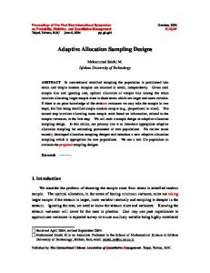
A virtual controller τc that stabilizes the system (27) uniformly, globally and exponentially, for some physically limited yaw rate, is proposed in [19] and given by (33)

1 0.5 0 −0.5

3 2 3    J(u):= ki |ωi | ωi2 + ki2 ωi2 + qi δi2 −ς lg(−ωi + 18) i=1

i=1

3 2 2    −ς lg(ωi +18)−ς lg(−δi +35)−ς lg(δi +35),

0

100

200

R EFERENCES [1] D. Enns, “Control allocation approaches,” in Proc. AIAA Guidance, Navigation and Control Conference and Exhibit, Boston MA, 1998, pp. 98–108. [2] J. M. Buffington, D. F. Enns, and A. R. Teel, “Control allocation and zero dynamics,” J. Guidance, Control and Dynamics, vol. 21, pp. 458–464, 1998. [3] O. J. Sørdalen, “Optimal thrust allocation for marine vessels,” Control Engineering Practice, vol. 5, pp. 1223–1231, 1997. [4] M. Bodson, “Evaluation of optimization methods for control allocation,” J. Guidance, Control and Dynamics, vol. 25, pp. 703–711, 2002. [5] O. H¨arkeg˚ard, “Efficient active set algorithms for solving constrained least squares problems in aircraft control allocation,” in Proc. IEEE Conf. Decision and Control, Las Vegas NV, 2002. [6] Y. Luo, A. Serrani, S. Yurkovich, D. Doman, and M. Oppenheimer, “Model predictive dynamic control allocation with actuator dynamics,” In Proceedings of the 2004 American Control Conference, Boston, MA, 2004. [7] ——, “Dynamic control allocation with asymptotic tracking of timevarying control trajectories,” In Proceedings of the 2005 American Control Conference, Portland, OR, 2005.

ηe2 [m]

Fig. 2.

400

500

600

Desired (dashed) and actual ship positions (solid).

10

ω

1 [Hz]

5 0 −5 −10 −15

2 [Hz]

20

ω

By investigating the given specifications of the system we can see that the Assumption 3 is also satisfied locally, since u is bounded. The gain matrices are chosen as follows: Kp := M · diag(3.13, 3.13, 12.5)10−2 , Kd := M · diag(3.75, 3.75, 7.5)10−1 , KI := M · diag(0.2, 0.2, 4)10−3 , −4 diag (1, 1, 10), Auˆ := Axˆ := 10, Γx˜ := I9×9 , Γ−1 θ2 := 10 −3 2I5×5 , Γθ1 := 10 , Γη := diag(103 , 103 , 3) and Γ := −1  where HTθˆW Hθˆ + εI W := diag (1, 1, 1, 1, 1, 0.9, 0.9, 0.7) and ε := 10−9 . The thruster loss vector θ1 and θˆ1 are given in Figure 6, θ2 := (0.05, 0.08, 0.02) and θˆ2 are given in Figure 7. The simulation results are presented in the Figures 28. The control objective is satisfied and the commanded virtual controls are tracked by the forces generated by the adaptive control allocation law: see Figure 5. Note that there are some deviations since ω saturates from 0 − 230s and since the loss parameter has changed at ca. 420s. Also note that the parameter estimates θˆ1 only converge to the true values when the ship is moving and the thrust loss is not zero. The simulations are carried out in a discrete MATLAB environment with a sampling rate of 20Hz

300

t [s]

,

10

0

−10 20

3 [Hz]

ki2 = 10

−3

ω

k3 = 0.02,

0 −0.05 −0.1

i=1

10 0 −10 −20

0

100

200

300

400

500

600

500

600

t [s] Fig. 3.

Actual propeller velocities

10

5

1 [deg]

ς = 0.05, k1 = k2 = 0.01, q1 = q2 = 2500.

0.1 0.05

0

δ

i=1

0

0.15

−5

−10 15 10

2 [deg]

i=1

1 0.5

−0.5

δ

i=1

1.5

ηe3 [deg]

where (27) is augmented with the integral action described by, ξ˙ = ηe . Thus Assumption 2 concerning high- and lowlevel control is satisfied. The cost function designed for the optimization problem, (5), is:

5 0 −5 −10 −15

0

100

200

300

400

t [s] Fig. 4.

Actual rudder deflection

0.2

0.1

0.1

1 [N]

0

loss

τ1 [N]

0.05

−0.05

0 −0.1

−0.1 −0.2

−0.15

0.2

0.3

0.1

2 [N]

0.1

loss

τ2 [N]

0.2

0 −0.1

0 −0.1 −0.2 −0.3

−0.2

3 [Nm]

0

loss

τ3 [Nm]

0.05

−0.05 −0.1

−3

20

0.1

15 10 5 0 −5

0

100

200

300

400

500

600

x 10

0

100

200

Fig. 5. The virtual control (dashed) and actual (solid) forces generated by the actuators

0.6

θ11

0.4 0.2 0 −0.2 0.6

θ12

0.4 0.2 0 −0.2 −3 x 10 2

θ13

1.5 1 0.5 0

0

100

200

300

400

500

600

t [s] Fig. 6.

Actual (dashed) and estimated (solid) loss parameters

0.06

θ

21

0.04

0.02

0 0.1

θ

22

0.08 0.06 0.04 0.02 0 0.025

θ23

0.02 0.015 0.01 0.005 0

0

100

200

300

400

t [s] Fig. 7.

Effector model parameter estimates

500

600

300

400

500

600

t [s]

t [s] Fig. 8.

Actual thrust loss

[8] V. Poonamallee, S. Yurkovich, A. Serrani, D. Doman, and M. Oppenheimer, “Dynamic control allocation with asymptotic tracking of timevarying control trajectories,” In Proceedings of the 2004 American Control Conference, Boston, MA, 2005. [9] T. A. Johansen, T. I. Fossen, and S. P. Berge, “Constrained nonlinear control allocation with singularity avoidance using sequential quadratic programming,” IEEE Trans. Control Systems Technology, vol. 12, pp. 211–216, 2004. [10] T. A. Johansen, T. I. Fossen, and P. Tøndel, “Efficient optimal constrained control allocation via multi-parametric programming,” AIAA J. Guidance, Control and Dynamics, vol. 28, pp. 506–515, 2005. [11] T. A. Johansen, “Optimizing nonlinear control allocation,” Proc. IEEE Conf. Decision and Control. Bahamas, pp. 3435–3440, 2004. [12] J. Tjønn˚as and T. A. Johansen, “Adaptive optimizing nonlinear control allocation,” In Proc. of the 16th IFAC World Congress, Prague, Czech Republic, 2005. [13] ——, “On optimizing nonlinear adaptive control allocation with actuator dynamics,” 7th IFAC Symposium on Nonlinear Control Systems, Pretoria, South Africa, 2007. [14] J. Tjønn˚as, A. Chaillet, E. Panteley, and T. A. Johansen, “Cascade lemma for set-stabile systems,” 45th IEEE Conference on Decision and Control, San Diego, CA, 2006. [15] A. Teel, E. Panteley, and A. Loria, “Integral characterization of uniform asymptotic and exponential stability with applications,” Maths. Control Signals and Systems, vol. 15, pp. 177–201, 2002. [16] Y. Lin, E. D. Sontag, and Y. Wang, “A smooth converse lyapunov theorem for robust stability,” SIAM Journal on Control and Optimization, vol. 34, pp. 124–160, 1996. ˚ [17] A. J. Sørensen, A. K. Adnanes, T. I. Fossen, and J. P. Strand, “A new method of thruster control in positioning of ships based on power control,” Proc. 4th IFAC Conf. Manoeuvering and Control of Marine Craft, Brijuni, Croatia,, 1997. [18] T. I. Fossen and M. Blanke, “Nonlinear output feedback control of underwater vehicle propellers using feedback form estimated axial flow velocity,” IEEE Journal of Oceanic Engineering, vol. 25, no. 2, pp. 241–255, 2000. [19] K. P. Lindegaard and T. I. Fossen, “Fuel-efficient rudder and propeller control allocation for marine craft: Experiments with a model ship,” IEEE Trans. Control Systems Technology, vol. 11, pp. 850–862, 2003. [20] L. Pivano, T. A. Johansen, Ø. N. Smogeli, and T. I. Fossen, “Nonlinear Thrust Controller for Marine Propellers in Four-Quadrant Operations,” American Control Conference (ACC), New York, USA, July 2007. [21] L. Pivano, Ø. N. Smogeli, T. A. Johansen, and T. I. Fossen, “Marine propeller thrust estimation in four-quadrant operations,” 45th IEEE Conference on Decision and Control, San Diego, CA, USA, 2006.