Optimizing Energy-Latency Trade-off in Sensor Networks with ...

Optimizing Energy-Latency Trade-off in Sensor Networks with Controlled Mobility Ryo Sugihara

Rajesh K. Gupta

Computer Science and Engineering Department University of California, San Diego La Jolla, California 92093 Email: {ryo, rgupta}@ucsd.edu

Abstract—We consider the problem of planning path and speed of a “data mule” in a sensor network. This problem is encountered in various situations, such as modeling the motion of a data-collecting UAV in a field of sensors for structural health monitoring. Our specific context here is use of a data mule as an alternative or supplement to multihop forwarding in a sensor network. While a data mule can reduce the energy consumption at each sensor node, it increases the latency from the time the data is generated at a node to the time the base station receives it. In this paper, we introduce the “data mule scheduling” or DMS framework that enables data mule motion planning to minimize the data delivery latency. The DMS framework is general; it can express many previously proposed problem formulations and problem settings related to data mules. We design algorithms for DMS and extend to the more general case of combined data mule and multihop forwarding to enable a flexible trade-off between energy consumption and data delivery latency. Using DMS, we can calculate the optimal way for node-to-node forwarding and data mule motion plan. Our implementation and simulation results using ns2 show nearly monotonic decrease of data delivery latency for greater limits on the energy consumption, thus vastly increasing the flexibility in the energy-latency trade-off for sensor network communications.

I. I NTRODUCTION Controlled mobility presents an attractive alternative to multihop forwarding for efficient data collection in a sensor field. In particular, we consider collecting data from stationary sensor nodes using a “data mule” via wireless communication. A data mule is a mobile node with radio and sufficient amount of storage to store the data from the sensors in the field. Data mules have been used in recent sensor network applications, e.g., a robot in underwater environmental monitoring [1] and a UAV (unmanned aerial vehicle) in structural health monitoring [2]. A data mule travels across the sensor field and collects data from each sensor node when the distance is short, and later deposits all the data to the base station. In this way, each sensor node can conserve energy, since it only needs to send the data over a short distance and has no need to forward other sensors’ data all the way to the base station. Note that energy issue is critical for sensor nodes as opposed to the data mule that returns to the base station after the travel. However, one disadvantage of this approach is that it generally takes more time to collect data, which in turn incurs larger data delivery latency. Thus optimizing the data delivery latency is vital for the data mule approach to be useful in practice.

In this paper, we study the problem of optimizing the energy-latency trade-off when using a data mule. We design a problem framework for optimizing the data mule’s movement, which we call the data mule scheduling (DMS) problem, and extend it to a general problem that combines data mule and multihop forwarding. Compared to previous studies, the DMS framework is comprehensive and general in the sense that it is capable of expressing many other formulations. It is also flexible enough to adapt to different problem settings. In the DMS problem setting, we can control the movement of the data mule (path, speed) as well as its communication (i.e., from which node it collects data at certain time duration). There is some similarity to classical scheduling problems. For instance, the communication between the data mule and each node can be represented as a job that has both time and location constraints. We analyze and design algorithms for the case that each sensor node generates data periodically. This applies to many sensor network application scenarios that monitors the field in the long term and thus enlarges the applicability of the DMS framework. Then we consider the combined approach of data mule and multihop forwarding. In the pure data mule approach, the energy consumption at each node is minimum and the data delivery latency is relatively large. On the other hand, multihop forwarding requires greater energy due to increased data transfer at each node but the latency is expected to be much shorter. Our work combines these two approaches in such a way that the designers of sensor networks can balance the energy consumption and the data delivery latency according to application needs. We formulate the problem by extending the DMS problem and design centralized and distributed algorithms. Then we implement the combined approach on the ns2 network simulator [3] to experimentally evaluate the effectiveness of the formulation and algorithms. Our contributions are: • Formulate the DMS problem, a problem framework for optimal control of data mule for minimizing the data delivery latency; • Analyze the DMS problem for the periodic data generation case; • Extend the DMS problem for the combined approach of data mule and multihop forwarding for a flexible control of the energy-latency trade-off, and design centralized and

2

distributed algorithms for the extended DMS problem; Demonstrate the effectiveness of formulation and algorithms by experiments on ns2 network simulator. The rest of this paper is organized as follows. In Section II we introduce related work. Section III gives an overview of the DMS problem. In Section IV we design algorithms for periodic data generation case in the DMS problem. Section V discusses the combined approach of data mule and multihop forwarding for the extended DMS problem. The centralized algorithm based on linear program formulation is also presented. Section VI describes the distributed algorithm for the forwarding problem. Section VII shows the results of the simulation experiments on ns2 network simulator and Section VIII concludes the paper. •

II. R ELATED W ORK Use of mobile nodes for data collection have been explored in sensor networks. Somasundara et al. [4], [5] studied the problem of choosing the path of a data mule that traverses at a constant speed through a sensor field with sensors generating data at a given rate. Their formulation also requires the data mule to visit the exact location of each sensor to collect data. They designed heuristic algorithms (based on EDF scheduling) to find a path that minimizes the buffer overflow at each sensor node. In the Message Ferrying project, Zhao and Ammar [6] examined the problem of path and speed optimization of a data mule in a field of stationary nodes. The project has extended the work on controllably mobile nodes case [7], multiple data mules case [8], and arbitrarily mobile nodes case [9]. While these formulations are similar in spirit to ours, we also generalize the problem to include a precise mobility model with acceleration constraints and stronger guarantees on the optimality, as demonstrated in our previous study [10]. There are also studies on combined data mule and multihop forwarding approach. Ho and Fall [11] discussed such approach in the context of Delay Tolerant Networking (DTN) architecture. Burns et al. [12] experimentally showed that controlled mobility can improve performance of routing in a network of randomly mobile nodes. Also relevant to this paper is work by Kansal et al. [13], who studied the case in which a data mule periodically travels across the sensor field along a fixed path. In their model, they can only change the speed of data mule. They used directed diffusion [14] for collecting data from the nodes outside of the direct communication range of the data mule. Their focus is on designing a robust communication infrastructure that works even in uncertain environments. Our work builds upon this work and seeks to build a formal understanding of the problem with stronger guarantees on the results. Ma and Yang [15], [16] designed a heuristic algorithm for path selection of a data mule. They formulate the multihop forwarding problem as a max-flow problem, assuming there is a limit on energy consumption at each node. Their formulation is similar to ours in some ways, but one of the limitations is that their path selection algorithm can be applied only for certain types of configurations. Specifically, they assume that

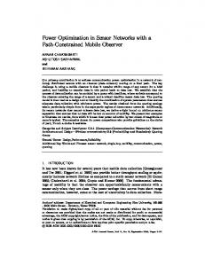
a data mule starts from the left edge of the deployment area, moves toward the right edge, and comes back to the left edge again. The algorithm also works only for connected networks. Xing et al. [17] also designed path selection algorithms when each node can forward data toward the base station along a routing tree constructed in advance. Their formulation is similar to the traveling salesman problem (TSP). They also assume the existence of a different type of nodes that do not generate data by themselves, in order to make the network connected and enable the construction of routing tree rooted at the base station. Although these assumptions allow the failover mechanism that improves the data delivery rate, they also limit the applicability of the technique. Our problem framework can express not only their settings, but also more general settings including disconnected networks. III. P ROBLEM F RAMEWORK FOR O PTIMAL C ONTROL OF DATA M ULE To control a data mule for data collection, one needs to determine the path and speed of the data mule and the schedule (i.e., when to collect data from a node). However, simultaneously optimizing them is an NP-hard problem, which is implied by the NP-hardness of the simplified path selection problem [10]. Consequently, in previous studies, the problem has been simplified in various ways by employing assumptions that restrict the capabilities of sensor nodes and data mule. Some examples are: data collection is only possible at the exact location of each node, and the data mule can move only at a constant speed. These assumptions are sometimes appropriate, but often make the formulation only applicable to a specific application and setting. Our goal for designing the DMS problem is to provide a comprehensive and flexible problem framework in which we can fully exploit the networking and mobility capabilities. For this purpose, we first decompose the problem into following three subproblems (see Figure 1(b)(c)(d)): 1) Path selection: determines the trajectory of the data mule so that it travels within each sensor node’s communication range at least once. 2) Speed control: determines how the data mule changes the speed along the path, so that it spends enough time within each node’s communication range to collect all the data from it. 3) Job scheduling: determines the schedule of data collection from each node. The last two subproblems are solved jointly as a scheduling problem with both location and time constraints, which we call the 1-D DMS problem. As for the path selection subproblem, we have formulated it as an independent problem in [10], which we briefly describe later. The DMS problem stated above is general and can be used to express several earlier problems in the area. For instance, the assumption of no wireless communication (as in [4] [5]) is easily expressed by setting the communication range to zero in the path selection subproblem. The constant speed assumption

3

node B

node C

node A

Location job A B C

Execution time e(A) e(B) e(C) Location

Execution time e(A) e(B) e(C) Time

Speed A’ B’ C’

Data mule Communication range

(a) Forwarding

Job A’ B’ C’

Time

Time

(b) Path selection

(d) Job scheduling

(c) Speed control

1-D DMS Data Mule Scheduling (DMS)

Fig. 1. Subproblems of the DMS problem: Forwarding problem (discussed in Section V) formulates the combined approach of data mule and multihop forwarding.

(as in [15]–[17]) and variable speed assumption (as in [6], [13]) are handled in the speed control subproblem. In the following three sections, we discuss details of the DMS problem and how we extend it to broaden the coverage for more general cases. First, in Section IV, we analyze the general case of the 1-D DMS problem in which each sensor node generates data periodically. Then, in Section V, we consider the hybrid case that combines data mule with multihop forwarding. We realize this by adding the “forwarding” subproblem in front of the path selection subproblem, as shown in Figure 1(a). Finally in Section VI, we design a distributed algorithm for the forwarding subproblem. IV. P ERIODIC 1-D DMS P ROBLEM Once we choose a path of the data mule, or the data mule moves along a predetermined path, by considering the path as a location axis, we obtain the 1-D DMS problem. The problem consists of two subproblems: speed control and job scheduling. The input to the speed control subproblem is a set of location jobs representing data collection tasks. A location job has an execution time and is associated with (possibly multiple) location intervals that correspond to the intersections of the node’s communication range and the data mule’s path. A solution for the 1-D DMS problem is twofold. One is “time-speed profile,” which determines the speed changes of the data mule. With a time-speed profile, each point on the location axis can be mapped onto a point on the time axis. Then we obtain a scheduling problem having a set of jobs, each of which has an execution time and feasible intervals. For this problem, we need to determine “job schedule” that defines when the data mule communicates with each node. The objective of the 1-D DMS problem is to find a speed control plan and a feasible job schedule so that the total travel time of the data mule is minimized. In the periodic case of the 1-D DMS problem, each sensor node generates data at a given rate and a data mule travels across the sensor field periodically. This models a common type of sensor network applications that continuously monitors the field in the long term, and has a larger coverage than nonperiodic case, which has been analyzed in our previous work

[18]. The objective is to minimize the period, i.e., the time the data mule takes for each travel, since it largely affects the data delivery latency. In the speed control subproblem, we consider three different constraints on the dynamics of the data mule. The first is “constant speed,” where the data mule cannot change the speed after it starts to move. The second is “variable speed,” where the data mule can instantaneously change the speed within a speed range [vmin , vmax ]. The third is “variable speed with acceleration constraint,” which we call the “generalized” model, since it includes previous two models as special cases. In the generalized model, the data mule can change the speed, but the rate of change is within the maximum absolute acceleration amax . This model is most appropriate when we cannot ignore the inertia, for example in case that a helicopter is used as a data mule as in [2]. We now present the algorithms for the 1-D DMS problem under different dynamics constraints. A. Terminology, definitions, and assumptions For the job scheduling subproblem, a job τi has an execution time ei and a set Ii of feasible intervals. A feasible interval I ∈ Ii is a time interval [r(I), d(I)], where r(I) is a release time and d(I) is a deadline. A job can be executed only within its feasible intervals. A simple job is a job with one feasible interval, whereas a general job can have multiple feasible intervals. For instance, in Figure 1(d), job B’ and C’ are simple jobs and job A’ is a general job. Similarly for the speed control subproblem, a location job τi has an execution time ei and a set Ii of feasible location intervals. A feasible location interval I ∈ Ii is a location interval [r(I), d(I)], where r(I) is a release location and d(I) is a deadline location. A location job can be executed only within its feasible location intervals. A simple location job is a location job with one feasible location interval, whereas a general location job can have multiple feasible location intervals. In Figure 1(c), location job B and C are simple location jobs and location job A is a general location job. For an interval I = [r, d] (also for a location interval), |I| denotes the length d − r. We also define containment as

4

follows: I ⊆ I ′ if and only if r′ ≤ r and d ≤ d′ where I ′ = [r′ , d′ ]. Let Tt denote the travel time of one period. The data mule needs to stay at the base station for constant time Tb to deposit the data to the base station and refuel etc. Thus the length of one period is Tt + Tb . For the system to be stable, in each period of travel, the data mule needs to collect the data generated in one period. Each sensor node is stationary. Communication range and data generation rate are known. Communication is always successful in the communication range and bandwidth is a known constant. All location jobs are preemptible without any cost incurred and can be executed over multiple feasible location intervals. There is no dependency among the location jobs. There is only one data mule. Data mule can communicate with one node at a time. Depending on the dynamics constraint, data mule may have constraints on the maximum speed and maximum acceleration. B. Algorithms 1) Processor demand analysis: First we present an algorithm based on processor demand analysis. This algorithm applies to the constant speed model with simple location jobs, i.e., each location job has only one feasible location interval. Let ei denote the execution time of i-th location job for one period. It is defined as follows: λi (Tt + Tb ), (1) R where λi is the data generation rate of i-th node and R is the bandwidth, both of which are known constants. ProcessorP demand g(I) for location interval I for one period is g(I) ≡ Ii ⊆I ei , where Ii is the feasible location interval of the i-th location job. Let g ′ (I) denote the processor demand for I for unit time, which is defined as follows: X λi g(I) g ′ (I) ≡ = . (2) Tt + Tb R ei

≡

When Tb = 0, we obtain the following from (3): |I0 | ≤

v ≤ min

I⊆I0

|I| 1 |I| = min , g(I) Tt + Tb I⊆I0 g ′ (I)

(3)

where I0 is the total travel interval. When Tb > 0, we obtain the following constraint using Tt = |I0 |/v:   |I| 1 v ≤ min − |I0 | . (4) I⊆I0 g ′ (I) Tb For a feasible solution to exist, the following must be satisfied: |I0 |


0, we have zk zi = , (8) li+1 − li lk+1 − lk

Ii ⊆I

The set of location jobs is feasible if and only if the speed v of data mule satisfies

min

I⊆I0

•

•

where k is any value satisfying lk+1 − lk > 0. (Feasible interval) pij ≥ 0 if ∃I ∈ Ij , [li , li+1 ] ⊆ I, where Ij is the set of feasible location intervals of location job j. Otherwise pij = 0. (Job completion) For location job j, ! 2m+1 2m+1 X X λj pij = (9) zi + T b , R i=0 i=0

where R is the bandwidth of communication from each node to the data mule. The right hand side is the amount of time to transmit the P data generated in one period. • (Processor demand) j pij ≤ zi . The LP problem may be either infeasible or unbounded2 . When it is infeasible, it is impossible to collect all data. When it is unbounded, the speed is arbitrary.

1 A location interval degenerates to a point when l = l i i+1 , but it does not affect the validity of the formulation. 2 It may be unbounded only in the constant speed model.

5

3

3 2,3

3

1,

3

2,3,4

1, 2

1

5

s (Base station)

(a)

1

4

1,4

2,4 ,5 1, 5

4

1, 2

4

3, 4

2,

2

2

4,5 ,5 3,4

For the obtained solution, we can make a job schedule in the following way. Pi−1Location Pi interval [li , li+1 ] is mapped to the time interval [ k=0 zk , k=0 zk ]. For each time interval, we allocate pi1 for job 1 from the start of the interval, pi2 for job 2 after that, and continue this for all jobs. 3) Iterative method: For the generalized model, we have designed a heuristic algorithm for the non-periodic case in [18]. The algorithm assumes a speed control in which the data mule first accelerates at amax , then keeps the top speed, and decelerates at amax , and finds the maximum top speed that preserves the feasibility. Then it applies recursively to the location intervals that admit further increase of the speed. We can use this algorithm for periodic case as well. Specifically, we can estimate Tt iteratively in the following manner: • Run the LP-based algorithm assuming no acceleration constraint (i.e., the variable speed model). Set the result to the initial value of Tˆt , the estimate of Tt . • Repeat – Run the heuristic algorithm with the execution time ei = λi (Tˆt + Tb )/R. Denote the travel time as T˜t . – If |T˜t − Tˆt | < ǫ, break the loop. Otherwise, update Tˆt by T˜t and repeat.

1

5

5

s

(b)

Fig. 2. Path selection problem: (a) Original problem with an example path. (b) Simplified problem, in which the objective is to find the shortest labelcovering tour in the graph.

Using the DMS problem, we are able to determine data mule’s speed and schedule for sensor data collection so that the travel time is minimized. We now consider a combined approach of data mule and multihop forwarding. In our framework, we realize this by defining a new “forwarding” problem that is placed in front of the DMS problem as shown in Figure 1. The forwarding problem is to determine how much data each node forwards to other nodes and to the data mule while satisfying a predetermined energy consumption constraint. First we consider the path selection problem. Then we discuss the forwarding problem and present a centralized algorithm based on linear program formulation.

labels associated with it. The objective is to find a “labelcovering tour” that minimizes the total cost of the edges in the tour, where “label-covering” means that, for any label, there exists at least one edge in the tour that contains the label. We use Euclidean distance as the cost metric, since we have observed in the experiments that it has a strong positive correlation with the shortest travel time in the induced 1-D DMS problem. The simplified problem is still NP-hard and we have designed an approximation algorithm. The algorithm first finds a TSP tour by using any TSP solver as an external module. Then, using dynamic programming, it finds a short label-covering tour that can be constructed by shortcutting the TSP tour, which is also a label-covering tour by itself. The algorithm runs in CT SP + O(n3 ) time, where CT SP is the computation time of the TSP solver. An approximate label-covering tour TAP P found by this algorithm satisfies |TAP P | ≤ α(|TOP T |+ 2nr), where α is the approximation ratio of the TSP solver, TOP T is the shortest label-covering tour, n is the number of nodes, and r is the radius of communication range. Simulation experiments have demonstrated that our formulation and algorithm effectively exploit broader communication range and yield shorter travel time than previous studies such as [6], [15]–[17].

A. Overview of path selection problem

B. Forwarding problem

For the nodes to send their data to the data mule, a path needs to intersect with their communication ranges, as shown in Figure 2(a). The objective is to find a path such that the shortest travel time of the data mule in the 1-D DMS problem induced by that path is minimized. However, finding a “smooth” path as shown in the figure is computationally expensive. In addition, maneuvering the data mule along such a smooth path is often difficult in practice. From these reasons, we have designed and analyzed a simplified problem in [10]. As shown in Figure 2(b), we consider a complete graph having vertices at sensor nodes’ locations and assume the data mule moves between vertices along a straight line. Each edge is associated with a cost and a set of labels, where the latter represents the set of nodes whose communication ranges intersect with this edge. In this way, while traveling along an edge, the data mule can collect data from the nodes in the

The objective of the forwarding problem is to find a forwarding plan such that the induced DMS problem has the shortest total travel time. Different from the “pure” data mule approach, in which each node sends its data only to the data mule, it can now forward its data to other neighboring nodes as well. More importantly, if a node decides to forward all data to other nodes, the data mule does not need to collect data directly from this node. Then the data mule can possibly take a shorter path to reduce the travel time. We present a centralized algorithm based on linear program formulation. Since finding the optimal forwarding plan that minimizes the travel time in the induced DMS problem is at least as hard as the DMS problem, we make it an independent problem by changing the objective function. We minimize the average distance of nodes from the base station weighted by the amount of data at each node after

V. C OMBINING DMS WITH M ULTIHOP F ORWARDING

6

forwarding. There are three reasons why this is a reasonable choice as the objective function. First, this function is likely to shorten the path of the data mule by forcing the nodes at the edge of network to primarily use forwarding. Secondly, this function allows a smooth transition between the data mule approach and multihop forwarding. As the energy consumption limit grows, more data is forwarded closer to the base station. In a connected network, all the data is eventually forwarded to the base station without using a data mule, which is equivalent to “pure” multihop forwarding. Finally, since the function is linear, we can formulate the problem as a linear program as described below. We assume the location of sensor nodes and the connectivity between them are known. We also assume the following parameters are given: • λi : Data generation rate of node i • Elimit : Energy consumption limit at each node per unit time • Er , Es : Energy consumption for receiving and sending unit data • R: Bandwidth, i.e., maximum data rate that each node can communicate with other nodes and the data mule Then we have the following linear program: Variables • xij : Amount of data sent from node i to j per unit time P ′ Objective Minimize i di λi , where di is the distance between node i and the base station, and λ′i is the data rate that node i sends directly to the data mule. λ′i is defined by the difference of incoming data rate and outgoing data rate as follows: X X λ′i = xji + λi − xij . (10) j

j

Constraints • xii = 0. • (Connectivity) For i 6= j, xij ≥ 0 if node j is in the communication range of node i. Otherwise xij = 0. ′ • (Flow conservation) λi ≥ 0. • (Energy consumption) For each node i,   X X (11) Er xji + λi  ≤ Elimit , xji + Es  j

j

•

where the first term in the left hand side is the amount of energy consumed by receiving data and the second term is that for sending data. About the latter, node i sends P ′ j xij to other nodes and λi to the data mule per unit time, when averaged overP time. Using Equation (10), the sum of these two equals j xji + λi . (Bandwidth) Per unit time, the amount of incoming data P P is j xji and outgoing data is j xij + λ′i . After some manipulations, we obtain X 2 xji + λi ≤ R. (12) j

The formulation above is also capable of expressing the case in which each node communicates along the preconstructed routing tree as in [17]. This is possible by replacing the connectivity constraint with the following one: • (Routing tree) For i 6= j, xij ≥ 0, if node j is node i’s parent in the routing tree. Otherwise xij = 0. VI. D ISTRIBUTED A LGORITHM FOR F ORWARDING The LP formulation above yields the optimal forwarding plan in the sense that it minimizes the weighted distance of data from the base station. However in practice, it may be difficult to tell each node about the list of forwarding destination and the data rate for each. To cope with this issue, we present a distributed algorithm where each node determines the forwarding destination and the data rate in a distributed manner. In the algorithm, we consider the case that each node forwards the data along a routing tree. For connected networks, there is only one routing tree rooted at the base station. For disconnected networks, there are multiple routing trees, one for each connected cluster. In each cluster, the node closest to the base station is chosen as the root. We describe how to identify connected clusters, construct intra-cluster routing trees, and plan the forwarding rate. A. Clustering and constructing routing trees We can simultaneously find connected clusters and construct intra-cluster routing trees by extending DSDV [19], which is a routing scheme based on the distance vector algorithm. We extend DSDV so that each node exchanges ID and position of the interim root node. An interim root node is the node that is reachable and closest to the base station as far as the current node knows. The information on root node is updated when the current node knows the one closer to the base station, and is propagated to neighbors when it is updated. These communications can be piggybacked on the update packets of normal DSDV. When it reaches a convergence, each node has the correct information on the root node and the next hop for reaching the root. To plan the forwarding rate, each node needs to learn the set of immediate child nodes as well as the parent. This is realized by each node sending a message to the parent node along the established routing tree. B. Planning the forwarding rate Forwarding rate is calculated in the following three phases. 1) Request: The request phase is initiated from the leaf nodes and proceeds toward the root. Each node tells the parent the cumulative data rate, which is the total data rate generated at the node and its descendants. Let Λi denote cumulative data rate of node i, which is defined as follows: X Λi ≡ λi + Λj , (13) j∈Ci

where Ci is the set of immediate children of node i.

7

2) Allocate: The allocate phase proceeds downwards from the root. Parent node tells each immediate child the allocated data rate, which is the maximum data rate that the parent can receive from this child. (in) Let yi denote the total data rate that node i receives from (in) its children. Then yi needs to satisfy (in)

Er y i

(in)

+ (λi + yi

)Es ≤ Elimit ,

Elimit − λi Es ≤ . E r + Es

(15)

For each child node, we distribute the maximum data rate proportionally by the cumulative data rate. Thus the maximum data rate Xj that child node j can send to the parent i is

1.5g 1.5g

g g

1.5g 1.5g

(14)

and thus (in) yi

g g

(a)

(b)

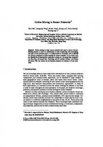
Fig. 3. Network topology: (a) Connected network; (b) Disconnected network. White circle is the base station. Line between two circles represents that they are within the communication range. Grid size g is set to 0.8r, where r is the radius of communication range, and a uniformly random disturbance of [−0.025r, 0.025r] is added to the position of each node.

We experimentally evaluate the combined approach of data mule and multihop forwarding in the periodic data generation case, specifically on the effectiveness of formulation and algorithms in optimizing the energy-latency trade-off.

period. If it is stable, we use the data for the next period as the final results. Figure 3 shows two network topologies we use for the experiments. Both of them have 100 sensor nodes, one base station and one data mule, but one is a connected network and the other is a disconnected network. The disconnected network consists of four connected networks of 25 nodes and the base station is not directly reachable from any nodes. For the data mule’s movement, we use the variable speed model. The range of speed is 0 ≤ v ≤ 10m/s, which roughly simulates the movement of a UAV used in [2]. For ns2 simulator, we use FreeSpace propagation model with 100m communication range. We use 802.11 MAC (with RTS/CTS) with 2 Mbps raw bandwidth, which is the default value for ns2. Packet size is 400 Bytes. Other parameters are set as follows. Energy consumption for sending/receiving unit data is assumed to be equal, i.e., Er = Es . The rate of data generation at each node λi is 100 Byte/sec. Let E denote the energy consumption at each node for “pure data mule” case without any node-to-node forwarding. Then E is expressed as λi Es , and this is the minimum possible value of Elimit . We measured the latency for Elimit = E, ..., 50E. Effective bandwidth R is set to 400 Kbps, considering the overhead of RTS/CTS and packet header.

A. Methods

B. Results

We have implemented the centralized and distributed algorithms for the forwarding problem and the algorithms for the DMS problem in MATLAB with YALMIP interface [20] and SeDuMi [21] for LP solver. The MATLAB program generates a Tcl script for ns2 [3], which simulates the movement of the data mule and the communication among the data mule and the nodes. To assess performance, we measure the delivery latency for each data packet from the time it is generated to the time the base station receives it either from neighboring nodes or via the data mule. For each test case, the simulation on ns2 is repeated multiple periods until it reaches stability. We consider it stable when the average delivery latency of the data received in the current period is within ±1% of that of the previous

Figure 4 is an example of forwarding plan and calculated path. The small circles represent the nodes and large circles are their communication ranges. Color of each circle represents how much data the node sends directly to the data mule. White circles mean zero and colored circles mean nonzero. As the forwarding algorithms try to gather data close to the base station, which is located in the center in this example, the nodes at the edge of the network forward all data to the ones closer to the center. Nodes that have the base station within their communication range forward all the data directly to the base station. In ns2 simulation, the delivery latency reached stability in all tested cases. Average number of periods until reaching stability was 5.2 (centralized) and 5.6 (distributed) in the

Elimit − λi Es . Λ Er + Es k k∈Ci

Xj = P

Λj

(16)

3) Plan: The plan phase proceeds upwards from the leaf nodes. Node determines the forwarding rate and tell it to the (out) parent. For node i, the total data rate yi to be sent to either the parent or the data mule is (out)

yi

(in)

= λi + yi

,

(17)

P (in) where yi = j∈Ci xji . We try to forward the data to parent node as much as possible and send the remaining data to the data mule. Therefore, if we let node j be the parent of i, data rate xij is o n (out) (18) xij = min yi , Xi . By setting xij in this way, inequality (15) is satisfied. Data rate λ′i to the data mule is (out)

λ′i = yi

− xij .

(19)

VII. S IMULATION E XPERIMENTS

8

500

Elimit = E

400 10 20 30 40 50 60 70 80 90 100

200

9

19 29

100

8

18 28 38 48 58 68 78 88 98

7 0 −100 −200 −300

39 49 59 69 79 89 99

17 27 37 47 57 67 77 87 97 1 26 36 46 56 66 76 86 96

6

16

5

15 25 35 45 55 65 75 85 95

4

14 24 34 44 54 64 74 84 94

3

13 23 33 43 53 63 73 83 93

2

12 22 32

42 52 62

72 82 92

−400 −500

0

500

Data delivery latency (sec)

11 21 31 41 51 61 71 81 91 101 300

Data mule only Avg latency = 432.81 sec

400 300

Elimit = 49 E Multihop forwarding only Avg latency = 4.17 sec

200 100 0

Fig. 4. Example of forwarding plan and calculated path: Connected network, Elimit = 10E, centralized forwarding algorithm. Nodes in white forward all data and the data mule does not collect data directly from them. Path is shown in bold line.

0

C. Discussions For both of the connected and the disconnected networks, the simulation results showed the decrease of data delivery latency as the energy consumption limit increases. The decrease was almost monotonic, demonstrating fine-grained control of the trade-off between energy and latency. It was also shown that formulation of the forwarding problem, especially the choice of objective function is appropriate, due to the fact that the centralized algorithm achieved a better trade-off than the distributed one, which yields suboptimal forwarding plans. We can also observe that the travel time of the data mule is nearly equal to the average latency for the data delivered by the data mule. It demonstrates that minimizing the travel time for the purpose of minimizing the data delivery latency is a valid approach. In addition, this implies that we can estimate the average delay solely by solving the DMS problem. Figure 7 shows the histograms of data delivery latency for two different energy consumption limits for each of the connected and disconnected networks. As these figures show,

Data delivery latency (sec)

600

connected network, and 4.0 (centralized) and 4.1 (distributed) in the disconnected network. Figure 5 shows the simulation results for the connected network and disconnected network when the centralized algorithm is used for the forwarding problem. For both networks, Elimit = E corresponds to the “pure data mule” case. The average latency in this case was 432.81 secs for the connected network and 513.07 secs for the disconnected network. These are quite similar to the total travel time (440.73 secs and 511.68 secs, respectively). For the connected network, it became “pure multihop forwarding” when Elimit = 49E, where all the data are sent to the base station by multihop forwarding and the data mule is not used. The average latency in this case was 4.17 secs. Figure 6 shows the comparison of average data delivery latency between the two forwarding algorithms. In both of the connected and disconnected networks, the centralized scheme based on LP formulation achieved shorter average latency than the distributed algorithm in most of the cases. On average, the ratio of average latency was 1.53 (min:0.93, max:2.05) for the connected network and 1.31 (min:0.95, max:1.80) for the disconnected network.

Avg latency (Base station) Avg latency (Data mule) Avg latency (Total) Data mule’s travel time

10

20 30 40 Energy consumption limit (×E ) Avg latency (Total) Data mule’s travel time

Elimit = E Data mule only Avg latency = 513.07 sec

500

50

400 300 200 100 0 0

10

20

30

40

50

Energy consumption limit (×E )

Fig. 5. Data delivery latency for varying energy consumption limit: (top) connected network, (bottom) disconnected network. The centralized forwarding algorithm is used.

regardless of the different network topology and the different total travel time, more than 98% of the data has delivery latency within double of the travel time. This means we can estimate the maximum delivery latency as well as the average. In practice, our problem formulation and algorithms provide sensor network designers a good estimate of the data delivery latency when there is an energy consumption limit, which is imposed by their application scenarios. Conversely, since the energy-latency curve is nearly monotonic and the problem is solved in relatively short time3 , by using binary search, we can also estimate the maximum energy consumption at each node when there is a constraint on the average or the maximum of data delivery latency, as assumed in [17]. VIII. C ONCLUSIONS AND F UTURE W ORK Controlled mobility, as represented by the motion of a data mule, provides an alternative approach to multihop forwarding for collecting data from sensor networks. While it allows a significant reduction in energy consumption, increased data delivery latency is a big issue. In this paper, we have presented the data mule scheduling (DMS) problem as a problem framework for optimally controlling a data mule and have extended it to enable flexible energy-latency trade-off. We have presented a framework to capture and analyze communication 3 For 100 nodes case, solving the forwarding problem and the DMS problem takes around 10 secs on MATLAB running on a PC.

9

(276.7)

400

Tt=234.08sec

100.00%

300 200

Tt=310.69sec

100

150

100

40

50

2Tt

99.98% 100

40

50

20

0

0 0

100

200

300

400

500

0

0 0

600

100

Data delivery latency (sec)

10

20

30

40

Connected network:

Energy consumption limit (× E ) 600

Size (KByte)

300 200 100

60 50 40

50

Fig. 6. Average data delivery latency for different forwarding algorithms: (top) connected network, (bottom) disconnected network

Elimit = 5E Cumulative dist. (%)

2Tt

100 80

99.25% 100

60 40

50

20 0 0

20 30 40 Energy consumption limit (× E )

600

Tt=137.33sec

80

0

0

500

150

100

100

98.20%

10

400

Disconnected network: Cumulative dist. (%)

2Tt

400

0

300

Data delivery latency (sec)

Elimit = 5E

(313.3) Tt=65.13sec

Centralized Distributed

500

200

50

Size (KByte)

0

100

200

300

400

500

600

Data delivery latency (sec)

Connected network:

80 60

20

100

Cumulative dist. (%) 100

150

80 60

0

Data delivery latency (sec)

Cumulative dist. (%)

2Tt

Size (KByte)

Centralized Distributed Size (KByte)

Data delivery latency (sec)

500

Elimit = 20E

20 0

0 0

100

200

300

400

500

600

Data delivery latency (sec)

Disconnected network:

Elimit = 20E

Fig. 7. Histogram of data delivery latency: For the connected network, gray bars are for the data delivered to the base station from neighboring nodes, and black bars are for the data delivered via the data mule. The centralized forwarding algorithm is used.

strategies that use combinations of data mule and multihop forwarding. To validate our results, we have implemented our algorithms and simulated them on ns2 network simulator. The results showed nearly monotonic decrease of the data delivery latency for larger energy consumption limit, demonstrating the effectiveness of the formulation and the algorithms in optimizing the energy-latency trade-off. Our future work includes making the problem formulation and the algorithms valid also in environments with increased uncertainty. For example, we are currently working on relaxing the assumption on communication region. One idea is to employ a “semi-online” algorithm that initially plans the motion offline solely based on the knowledge about small regions around each node. Then, at runtime, it opportunistically exploits the additional communication region that is not known beforehand to optimize the motion. R EFERENCES [1] I. Vasilescu, K. Kotay, D. Rus, M. Dunbabin, and P. Corke, “Data collection, storage, and retrieval with an underwater sensor network,” in SenSys, 2005, pp. 154–165. [2] M. Todd, D. Mascarenas, E. Flynn, T. Rosing, B. Lee, D. Musiani, S. Dasgupta, S. Kpotufe, D. Hsu, R. Gupta, G. Park, T. Overly, M. Nothnagel, and C. Farrar, “A different approach to sensor networking for SHM: Remote powering and interrogation with unmanned aerial vehicles,” in Proceedings of the 6th International workshop on Structural Health Monitoring, 2007. [3] “ns2 network simulator,” http://www.isi.edu/nsnam/ns/. [4] A. A. Somasundara, A. Ramamoorthy, and M. B. Srivastava, “Mobile element scheduling for efficient data collection in wireless sensor networks with dynamic deadlines,” in RTSS, 2004, pp. 296–305. [5] ——, “Mobile element scheduling with dynamic deadlines,” IEEE Trans. Mobile Computing, vol. 6, no. 4, pp. 395–410, 2007. [6] W. Zhao and M. Ammar, “Message ferrying: Proactive routing in highlypartitioned wireless ad hoc networks,” in FTDCS, 2003, pp. 308–314.

[7] W. Zhao, M. Ammar, and E. Zegura, “A message ferrying approach for data delivery in sparse mobile ad hoc networks,” in MobiHoc, 2004, pp. 187–198. [8] ——, “Controlling the mobility of multiple data transport ferries in a delay-tolerant network,” in INFOCOM, 2005, pp. 1407–1418. [9] M. M. B. Tariq, M. Ammar, and E. Zegura, “Message ferry route design for sparse ad hoc networks with mobile nodes,” in MobiHoc, 2006, pp. 37–48. [10] R. Sugihara and R. K. Gupta, “Improving the data delivery latency in sensor networks with controlled mobility,” in DCOSS, 2008. [11] M. Ho and K. Fall, “Poster: Delay tolerant networking for sensor networks,” in SECON, 2004. [12] B. Burns, O. Brock, and B. N. Levine, “MV routing and capacity building in disruption tolerant networks,” in INFOCOM, 2005, pp. 398– 408. [13] A. Kansal, A. A. Somasundara, D. D. Jea, M. B. Srivastava, and D. Estrin, “Intelligent fluid infrastructure for embedded networks,” in MobiSys, 2004, pp. 111–124. [14] C. Intanagonwiwat, R. Govindan, and D. Estrin, “Directed diffusion: a scalable and robust communication paradigm for sensor networks,” in MobiCom, 2000, pp. 56–67. [15] M. Ma and Y. Yang, “SenCar: An energy efficient data gathering mechanism for large scale multihop sensor networks.” in DCOSS, 2006, pp. 498–513. [16] ——, “SenCar: An energy efficient data gathering mechanism for largescale multihop sensor networks,” IEEE Trans. Parallel and Distributed System, vol. 18, no. 10, pp. 1476–1488, 2007. [17] G. Xing, T. Wang, Z. Xie, and W. Jia, “Rendezvous planning in mobilityassisted wireless sensor networks,” in RTSS, 2007, pp. 311–320. [18] R. Sugihara and R. K. Gupta, “Data mule scheduling in sensor networks: Scheduling under location and time constraints,” UCSD Tech. Rep., vol. CS2007-0911, 2007. [19] C. E. Perkins and P. Bhagwat, “Highly dynamic destination-sequenced distance-vector routing (DSDV) for mobile computers,” in SIGCOMM, 1994, pp. 234–244. [20] J. L¨ofberg, “Yalmip : A toolbox for modeling and optimization in MATLAB,” in Proceedings of the CACSD Conference, Taipei, Taiwan, 2004. [Online]. Available: http://control.ee.ethz.ch/∼joloef/yalmip.php [21] J. F. Sturm, “Using SeDuMi 1.02, a MATLAB toolbox for optimization over symmetric cones,” Optimization Methods and Software, vol. 11–12, pp. 625–653, 1999.