Optimizing Neural Networks with Kronecker-factored

Optimizing Neural Networks with Kronecker-factored Approximate Curvature Martens and Grosse, ICML 2015 Agustinus Kristiadi

SDA Reading Group, 25 May 2018

Outline Introduction Gradient Descent Natural Gradient Kronecker Product Kronecker Factored Approximate Curvature (K-FAC) Method Cost Results Conclusion References

Gradient Descent

I

Neural nets are mostly trained using gradient descent.

I

Gradient descent is first order method, so no curvature information.

Gradient Descent: Parametrization I

Gradient descent operates in Euclidean space with Euclidean metric.

I

Projecting complicated manifold in flat representation (left), which distort shape, distance, etc.

I

Training suffers from badly conditioned curvature.

Fisher Information Matrix I

Covariance of gradient of log-likelihood: F := E[∇θ log pθ ∇θ log pθ| ] = Cov(∇θ log pθ )

I

Equivalent to Hessian of KL-divergence of two distributions realizable by parameter θ and θ0 : F := ∇2θ0 DKL [pθ kpθ0 ]|θ0 =θ

I

Thus F gives curvature information in distribution space with KL-divergence as metric.

I

Second order Taylor series expansion of KL-divergence: 1 DKL [pθ kpθ0 ] ≈ (θ0 − θ)| F(θ0 − θ) 2

Natural Gradient

I

Second order method, similar to Newton’s method.

I

Use F instead of Hessian in the update θ = θ − αF−1 ∇θ pθ

I

Can be seen as ”adaptive learning rate”, which depends on the local curvature.

I

Independent to parameterization of θ. Only care about pθ itself.

Natural Gradient: Problem

I

Like Hessian, F is expensive: I I I

I

O(n2 ) storage. O(n3 ) inversion. n can be as high as 20M in VGGNet!

Needs an approximation! I

AdaGrad, RMSProp, Adam: diagonal Fisher approximation!

Kronecker Product

I

Let A ∈ Rm×n and B ∈ Rp×q .

I

Kronecker product is defined as:  a11 B · · ·  .. .. A⊗B= . . am1 B · · ·

I

A ⊗ B ∈ Rmp×nq .

 a1n B ..  . .  amn B

K-FAC

I

Consider l-th layer of a neural net with input al and output sl := Wl| al .

I

Weight gradient is given by: ∇Wl L = al (∇sl L)| = al gl| .

I

We have identity vec(uv | ) = v ⊗ u.

I

Approximate FIM of this layer’s weight with: Fl := E[vec(∇Wl L) vec(∇Wl L)| ] = E[gl gl| ⊗ al a|l ] ≈ E[gl gl| ] ⊗ E[al a|l ] =: Sl ⊗ Al

K-FAC: Assumption I I I

K-FAC: Fl ≈ E[gl gl| ] ⊗ E[al a|l ] K-FAC assumes independence between al and gl . If we assume further for each layer l, k with l 6= k, are independent. Then F is block diagonal constructed by Fl of each layer.

Figure: Exact F, K-FAC approximation, and their difference.

K-FAC: Inversion

I

Remember, in natural gradient we need to compute F−1 l ∇Wl L.

I

In K-FAC, Fl ≈ Sl ⊗ Al , so: −1 −1 F−1 l ∇Wl L = Sl ⊗ Al vec(∇Wl L) −1 = vec(A−1 l ∇Wl L Sl )

I

Thus we only need to store and invert the factors, instead of the full Fisher matrix!

K-FAC: Cost

I

Assume al ∈ Rn , sl ∈ Rm , and Wl ∈ Rn×m : I I I

I

Al ∈ Rn×n Sl ∈ Rm×m Space cost is thus O(n2 + m2 ) with inversion cost of O(n3 + m3 ).

Compare this to the cost of exact F: I I

F ∈ Rnm×nm Space cost in O(n2 m2 ), inversion cost in O(n3 m3 ).

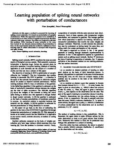
K-FAC: Results

Conclusion

I

Second order method has big benefit.

I

Natural gradient takes step in distribution space instead of parameter space.

I

Natural gradient is expensive, so needs approximation.

I

K-FAC assumes independence of layers in neural nets and use Kronecker product to factorize the Fisher Matrix.

I

Much cheaper than exact natural gradient, but still gives a lot of benefits.

References and Further Readings

I

Martens, James, and Roger Grosse. ”Optimizing neural networks with kronecker-factored approximate curvature.” International conference on machine learning. 2015.

I

Intro to natural gradient: https://wiseodd.github.io/ techblog/2018/03/14/natural-gradient/.