Jan 22, 2016 - geography Based Optimization for E-Mail Spam Identification. ... The email spam is commonly used for advertising products and services ...
Int. J. Communications, Network and System Sciences, 2016, 9, 19-28 Published Online January 2016 in SciRes. http://www.scirp.org/journal/ijcns http://dx.doi.org/10.4236/ijcns.2016.91002
Optimizing Feedforward Neural Networks Using Biogeography Based Optimization for E-Mail Spam Identification Ali Rodan, Hossam Faris, Ja’far Alqatawna King Abdallah II School for Information Technology, The University of Jordan, Amman, Jordan Received 26 December 2015; accepted 22 January 2016; published 25 January 2016 Copyright © 2016 by authors and Scientific Research Publishing Inc. This work is licensed under the Creative Commons Attribution International License (CC BY). http://creativecommons.org/licenses/by/4.0/
Abstract Spam e-mail has a significant negative impact on individuals and organizations, and is considered as a serious waste of resources, time and efforts. Spam detection is a complex and challenging task to solve. In literature, researchers and practitioners proposed numerous approaches for automatic e-mail spam detection. Learning-based filtering is one of the important approaches used for spam detection where a filter needs to be trained to extract the knowledge that can be used to detect the spam. In this context, Artificial Neural Networks is a widely used machine learning based filter. In this paper, we propose the use of a common type of Feedforward Neural Network called MultiLayer Perceptron (MLP) for the purpose of e-mail spam identification, where the weights of this network model are found using a new nature-inspired metaheuristic algorithm called Biogeography Based Optimization (BBO). Experiments and results based on two different spam datasets show that the developed MLP model trained by BBO gets high generalization performance compared to other optimization methods used in the literature for e-mail spam detection.
Keywords Spam, BBO, Multilayer Perceptron, Optimization, Biogeography Based Optimization
1. Introduction Spam can be defined as a form of unwanted communications usually sent in a large volume that negatively affects networks bandwidth, servers storage, user time and work productivity [1]-[4]. In the context of the internet, spammers utilize several applications including email systems, social network platforms, web blogs, web forums and search engines [5]. The email spam is commonly used for advertising products and services typically related How to cite this paper: Rodan, A., Faris, H. and Alqatawna, J. (2016) Optimizing Feedforward Neural Networks Using Biogeography Based Optimization for E-Mail Spam Identification. Int. J. Communications, Network and System Sciences, 9, 19-28. http://dx.doi.org/10.4236/ijcns.2016.91002
A. Rodan et al.
to adult entertainment, quick money and other attractive merchandises [6]. It is estimated that, in a single affiliate program, spammer revenue can exceed one million dollars per month [7]. Moreover, statistics show that there is a trend toward criminalizing commercial spam. The percentage of spam containing malicious contents increased compared to the one advertising legitimate products and services [8]. Several attacks such as phishing, cross-site scripting, cross-site request forgery and malware infection utilize email spam as part of their attack vectors [9]. The focus of this paper is on email spam as it is a common form of spam. Spam detection is considered a hard and challenging task. It is based on the assumption that the spam’s content differs from that of a legitimate email in ways that can be quantified. However, accuracy of the detection is affected by several factors including the subjective nature of spam, obfuscation, language issues, processing overhead and message delay, and the irregular cost of filtering errors [10]. Two approaches can be used for spam detection; rule-based filtering and learning-based filtering. In rules-based filtering, different parts of the messages such as header, content and source address are analyzed in order to define patterns and build a database of detection rules. Received email message is checked against these rules, and if a pattern matching of the rules is found, the message is classified as a spam. This approach needs a large number of rules to be affective. Nevertheless, rule-based filter could be evaded by forging the source of email and/or disguising the mail content [3] [10]. Alternatively, spam can be detected using learning-based filter. Such filter needs to be trained to extract the knowledge that can be used to detect the spam. This requires a large email dataset with both spam and legitimate ones. Most of these filters use Machines Learning (ML) algorithms such as Naive Bayes Classifier [11], Support Vector Machines [12] and Artificial Neural Networks [1]. Moreover, several ML techniques are combined together to produce a more accurate and robust detection methods [13]-[15]. For instance, Artificial Neural Network (ANN) is a commonly used technique as it gives accurate classification results [4] [13] [14] [16] [17]. ANNs are inspired by the biological neural systems. The most popular and applied type of ANNs is the Feedforward Multilayer Perceptron (MLP). MLP is a model that requires a considerable time for parameter selection and training [18] which has encouraged researchers to optimize it in several ways. Conventionally, MLP networks are optimized by gradient based techniques like the Backpropagation algorithm. However, gradient based techniques suffer some main drawbacks like the slow convergence, high dependency on the initial parameters and the high probability of being trapped in local minima [19]. Therefore, many researchers proposed stochastic methods for training MLPs which are based on generating a number of random solutions to solve the problem. One type of stochastic methods that is getting more interest in training neural networks is the nature-inspired metaheuristic algorithms. Examples of this type of algorithms are the Genetic Algorithm (GA) [16], Particle Swarm Optimization (PSO) [15], Differential Evolution (DE) [20] and Ant Colony Optimization (ACO) [21]. In the context of spam detection, the authors in [16] suggested to train MLP networks with Genetic Algorithm to optimize its performance in identifying spam. Their results show that such hybridized method outperform traditional MLP neural network. In this paper, we develop an MLP neural network model trained with the Biogeography based Optimization (BBO) [22] for identifying e-mail spam. BBO is a recent metaheuristic algorithm inspired by the biogeography natural process. In the literature, BBO proved high efficiency in training neuro-fuzzy networks [23] and MLP networks [24]. In this work, MLP is trained using BBO based on two different spam datasets and compared with other MLPs trained with the Backpropagation algorithm and common metaheuristic algorithms: GA, PSO, DE and ACO. This paper is organized as follows: Section 2 gives a broad description of Multilayer Perceptron (MLP) Neural Networks; Section 3 introduces and exposes how to perform Biogeography based optimization (BBO); BBO for training MLP is described in Section 4; The Datasets are described in Section 5; Section 6 exposes the experiments and analyzes the results obtained; and finally, Section 7 outlines some conclusions.
2. Multilayer Perceptron Neural Networks The human brain has the ability to perform multi-tasking. These tasks include several activities such as controlling the human body temperature, controlling blood pressure, heart rate, breathing, and other tasks that enable human beings to see, hear, and smell. The brain can perform these tasks at a rate that is far less than the rate at which the conventional computer can perform the same tasks [25]. The cerebral cortex of the human brain contains over 20 billion neurons with each neuron linked with up to 10,000 synaptic connections [25]. These neu-
20
A. Rodan et al.
rons are responsible for transmitting nerve signals to and from the brain. Very little is known about how the brain actually works but there are computer models that try to simulate the same tasks that the brain carries out. These computer models are called Artificial Neural Networks, and the method by which the Neural Network is trained is called a Learning Algorithm, which has the duty of training the network and modifying weights in order to obtain a desired response. The neuron (node) of a neural network is made up of three components: 1. synapse (connection link) which is characterised by its own weight, 2. An adder for summing the input signal, which is weighted by the synapse of the neuron, and 3. An activation function to compute the output of this neuron. The main Neural Network architectures are Feedforward Neural Network (FFNN) and the Recurrent Neural Network (RNN). The most common and well-known Feedforward Neural Network (FFNN) model is called Multi-Layer Perceptron (MLP). Let a MLP with K input units, N internal (hidden) units, and L output units, where
s = ( s1 , s2 , , sK ) , x = ( x1 , x2 , , xN ) , and y = ( y1 , y2 , , yL ) , be the inputs of the input nodes, the outputs of the hidden nodes, and outputs of the output nodes respectively. b j and bl are the biases in the input and T
T
T
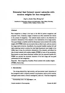
output layers. A three layer MLP is shown in Figure 1. In the forward pass, the activations are propagated from the input layer to the output layer. The activations of the hidden nodes are the weighted inputs from all the input nodes plus the bias b j . The activation of the jth hidden node is denoted as net j , and computed according to: K
∑V ji si + b j ,
= net j
(1)
i =1
In the hidden layer, the corresponding output of the jth node (e.g. x j ) is usually calculated based on a sigmoid function as follows:
xj =
1
(1 + e ) − net j
,
(2)
The outputs of the hidden layer ( x1 , x2 , , xN ) are used as inputs to the output layer. The activation of the output nodes ( y1 , y2 , , yL ) is also defined as the weighted inputs from all the hidden nodes plus the bias bl , where Wlj is the connection weight from the jth hidden node x j to the lth (linear) output node:
= yl
N
∑Wlj x j + bl , j =1
Figure 1. An example of the topology of the Multi-Layer Perceptron—MLP.
21
(3)
A. Rodan et al.
The backward pass starts by propagating back the error between the current output yl and the teacher output yˆl in order to modify the network weights and the bias values. The classical MLP network is attempted to minimise the Error (E) via the Backpropagation (BP) training algorithm [26], where for each epoch the Error (E) is computed as: = E
P
L
∑∑ yle − yˆle
2
,
(4)
=e 1 =l 1
where P is the number of patterns. In MLP all the network weights and bias values are assigned random values initially, and the goal of the training is to find the set of network weights that cause the output of the network to match the teacher values as closely as possible. MLP has been successfully applied in a number of applications, including regression problems [27], classification problems [28], or time series prediction using simple auto-regressive models [29].
3. Biogeography Based Optimization Biogeography based optimization (BBO) is an evolutionary computation algorithm motivated by a natural process (biogeography) which originally introduced by Dan Simon in 2008 [28]. BBO typically optimizes a multidimensional real-valued function by improving candidate solutions with regards of a given measurement or fitness function. It optimizes a given problem by combining an existing population of candidate solution with a newly created candidate solution according to a simple formula. In this way the objective function is behaving as a black box model that provides a measure of quality (fitness function) given a candidate solution [22]. The environment of BBO is analogous to an archipelago of islands, where each island is considered as a possible solution to the problem [30]. There are decision variables that is called suitability index variables (SIVs), where each island consists of SIVs. The performance is measured for each island by an objective function, where in our case we will use the habitat suitability index (HSI) for performance level measurement. BBO algorithm tries to randomly create new SIVs by using migration that shares the same SIVs with mutation [30]. The BBO algorithm can be described by the following steps [30]. 1. Define BBO parameters including the mutation probability and the elitism parameter as the same way as any genetic algorithms (GAs). 2. Initialize the population. Again, as the same way as any genetic algorithms (GAs). 3. Calculate the immigration and the emigration rates for each island, where good solution have a maximum emigration rate and minimum immigration rate, while bad solutions have a maximum immigration rate and minimum emigration rate. 4. Choose the immigrating islands based on the immigration rates. 5. Migrate randomly selected independent solution variables (SIVs) based on the previously selected islands. 6. Perform mutation for each island. 7. Replace the worst islands in the population with the newly generated islands. 8. If the termination condition is met, terminate; otherwise, go to step 3. BBO has been associated with several evolutionary computation algorithms, including particle swarm optimization [31], evolution strategy [32], harmony search [33], and case-based reasoning [34]. Moreover it has been extended to noisy [35] and multi-objective functions [36], and has been mathematically evaluated using Markov chain [37] and dynamic system [38] models.
4. BBO for Training MLP In our work the BBO algorithm is used for optimizing MLP network as follows: 1. A predetermined number of Habitats is generated. Each Habitat represents a set of weights of an MLP network. Therefore a Habitat corresponds to one MLP network. 2. The fitness value of the generated candidate networks in step 1 is calculated. In our implementation we use the Mean Squared Error (MSE). The goal is to minimize the difference between the actual and estimated values. The set of weights are assigned to an MLP network and the MSE (HSI) is calculated based on the training dataset. 3. Update emigration, immigration and mutation rates as described in the previous section. 4. MLP networks are combined, selected and mutated.
22
A. Rodan et al.
5. Some MLP networks with high fitness (low MSE value) are kept intact and passed to the next generation. 6. Steps 2 to 5 are repeated until the predetermined number of iterations is reached. The best MLP with the lowest MSE value is tested and evaluated on a separated unrepresented dataset. The whole process is shown in Figure 2.
5. Datasets In order to assess the BBO-MLP approach in identifying e-mail spam, we apply it on two different datasets. The first dataset is extracted from SpamAssassin public mail corpus1. This data consist of 9346 records with 90 features. Each example in the data is labeled as Ham or Spam. The data includes 6951 ham emails and 2395 spam emails. The percentage of spam email forms approximately 25.6% of the emails which makes the data imbalanced and therefore more challenging. The full description of the features can be found in [9]. The second dataset is obtained from the University of California at Irvine (UCI) Machine Learning Repository2 [39]. This data is consisted of 4601 instances and 57 features. Approximately 39.4% of the emails in this data are spam e-emails. The collected features in this data are based on frequency of some selected words and special characters in the e-mails.
6. Experiments and Results The developed BBO-MLP classifier is evaluated using the two datasets described in the previous section and compared with Genetic Algorithm (GA), Particle Swarm Optimization (PSO), Differential Evolution (DE), Ant Colony Optimization (ACO) and Back Propagation (BP) algorithms. All algorithms including BBO are tuned as listed in Table 1. For all metaheuristic algorithms the number of individuals in the population and number of iterations are unified. Each individual represents the connection weights of the neural network that connect the input layer to the hidden layer, the weights from the hidden layer to the output layer and the set of bias terms. In our experiments, we tried different numbers of neurons in the hidden layer of the trained networks: 5, 10 and 15 neurons respectively. Both datasets are equally split into two parts: one is used for training and the other is used for testing. Each experiment was repeated 10 times in order to get statistically significant results. Figure 3 and Figure 4 show the convergence curves for the metaheuristic algorithms based on the Spambase and SpamAssassin datasets respectively. It can be noticed in the figures that the BBO trainer has achieved the fastest and lowest convergence curves while GA and PSO come second and ACO is the worst. For each one of the training algorithms (GA, PSO, DE, ACO, BP, and BBO), we find the best representative MLP model and then evaluate it based on the accuracy rate, which is the number of correctly classified instances
Figure 2. Training MLP network using BBO. 1
https://spamassassin.apache.org/publiccorpus/ http://archive.ics.uci.edu/ml/
2
23
A. Rodan et al.
(a)
(b)
(c)
Figure 3. Convergence curves of BBO, GA, PSO, DE and ACO in training the MLP neural network with 5, 10 and 15 neurons in the hidden layer respectively for the Spambase dataset. (a) MLP-5; (b) MLP-10; (c) MLP-15. Table 1. Parameters settings of the metaheuristic algorithms. Algorithm
Parameter
Value
BBO
• Minimum wormhole existence probability
0.2
• Maximum wormhole existence probability
1
• Crossover probability
0.9
GA
PSO DE ACO
• Mutation probability
0.1
• Selection mechanisim
Stochastic universal sampling
• Acceleration constants
[2.1,2.1]
• Intertia weights
[0.9,0.6]
• Crossover probability
0.9
• Differential weight
0.5
• Initial pheromone (τ)
1e−06
• Pheromone update constant (Q)
20
• Pheromone constant (q) • Global pheromone decay rate ( pg )
1 0.9
• Local pheromone decay rate ( pt )
0.5
• Pheromone sensitivity (α)
1
• Visibility sensitivity (β)
5
24
A. Rodan et al.
(a)
(b)
(c)
Figure 4. Convergence curves of BBO, GA, PSO, DE and ACO in training the MLP neural network with 5, 10 and 15 neurons in the hidden layer respectively for the SpamAssassin dataset. (a) MLP-5; (b) MLP-10; (c) MLP-15.
divided by the total number of instances. Table 2 and Table 3 show the best, average and standard deviation values achieved by each approach for the Spambase and SpamAssassin datasets, respectively. According to the tables, it can be clearly seen that the BBO trainer achieved the highest averages and best accuracy rates results for both datasets (shown in bold fonts). It can be also noticed that 5 neurons in the hidden layer was good enough to train the MLP network. Most of metaheuristic trainers didn’t achieve any better results with the 10 and and 15 neurons in the hidden layer.
7. Conclusion In this work, a recent nature inspired metaheuristic algorithm named Biogeography Based Optimizer is used to train the Multilayer Perceptron neural network for the purpose of E-mail spam identification. The developed approach is evaluated and compared with four metaheuristic algorithms (GA, PSO, DE and ACO) and the gradient decent based Backpropagation algorithm. Two Spam datasets with their extracted features based on the content of the e-mails are deployed. The developed BBO based training approach showed significant improvement in the accuracy of identifying spam e-mails compared to the other approaches. The results of the experiments support the conclusion that BBO is very effective in avoiding local minima and have a relatively fast convergence
25
A. Rodan et al.
Table 2. Results of Spambase dataset. Number of neurons in the hidden layer 5 BBO
GA
PSO
DE
ACO
BP
10
15
Average
0.880
Average
0.879
Average
0.882
Stdv
0.011
Stdv
0.012
Stdv
0.012
Best
0.902
Best
0.892
Best
0.906
Average
0.858
Average
0.833
Average
0.833
Stdv
0.009
Stdv
0.011
Stdv
0.011
Best
0.873
Best
0.867
Best
0.902
Average
0.785
Average
0.785
Average
0.768
Stdv
0.019
Stdv
0.022
Stdv
0.009
Best
0.818
Best
0.812
Best
0.906
Average
0.681
Average
0.693
Average
0.708
Stdv
0.043
Stdv
0.037
Stdv
0.023
Best
0.740
Best
0.741
Best
0.751
Average
0.643
Average
0.623
Average
0.618
Stdv
0.043
Stdv
0.030
Stdv
0.065
Best
0.743
Best
0.671
Best
0.709
Average
0.658
Average
0.673
Average
0.720
Stdv
0.054
Stdv
0.060
Stdv
0.045
Best
0.747
Best
0.766
Best
0.787
Table 3. Results of SpamAssassin dataset. Number of neurons in the hidden layer 5 BBO
GA
PSO
DE
ACO
BP
Average
10 0.866
Average
Stdv
0.008
Best
0.880
Average
15 0.868
Average
0.866
Stdv
0.007
Stdv
0.006
Best
0.877
Best
0.875
0.830
Average
0.829
Average
0.830
Stdv
0.019
Stdv
0.019
Stdv
0.014
Best
0.863
Best
0.857
Best
0.855
Average
0.801
Average
0.795
Average
0.795
Stdv
0.006
Stdv
0.011
Stdv
0.010
Best
0.810
Best
0.810
Best
0.814
Average
0.772
Average
0.770
Average
0.770
Stdv
0.008
Stdv
0.014
Stdv
0.011
Best
0.783
Best
0.793
Best
0.785
Average
0.756
Average
0.751
Average
0.759
Stdv
0.008
Stdv
0.014
Stdv
0.012
Best
0.767
Best
0.768
Best
0.775
Average
0.775
Average
0.770
Average
0.786
Stdv
0.022
Stdv
0.016
Stdv
0.025
Best
0.807
Best
0.792
Best
0.824
26
A. Rodan et al.
toward the best solution.
References [1]
Guzella, T.S. and Caminhas, W.M. (2009) A Review of Machine Learning Approaches to Spam Filtering. Expert Systems with Applications, 36, 10206-10222. http://dx.doi.org/10.1016/j.eswa.2009.02.037
[2]
Rao, J.M. and Reiley, D.H. (2012) The Economics of Spam. The Journal of Economic Perspectives, 26, 87-110. http://dx.doi.org/10.1257/jep.26.3.87
[3]
Stern, H., et al. (2008) A Survey of Modern Spam Tools. CiteSeer.
[4]
Su, M.-C., Lo, H.-H. and Hsu, F.-H. (2010) A Neural Tree and Its Application to Spam E-Mail Detection. Expert Systems with Applications, 37, 7976-7985. http://dx.doi.org/10.1016/j.eswa.2010.04.038
[5]
Kanich, C., Weaver, N., McCoy, D. Halvorson, T., Kreibich, C., Levchenko, K., Paxson, V., Voelker, G.M. and Savage, S. (2011) Show Me the Money: Characterizing Spam-Advertised Revenue. USENIX Security Symposium, 15.
[6]
Cranor, L.F. and LaMacchia, B.A. (1998) Spam! Communications of the ACM, 41, 74-83. http://dx.doi.org/10.1145/280324.280336
[7]
Stone-Gross, B., Holz, T., Stringhini, G. and Vigna, G. (2011) The Underground Economy of Spam: A Botmaster’s Perspective of Coordinating Large-Scale Spam Campaigns. USENIX Workshop on Large-Scale Exploits and Emergent threats (LEET), Vol. 29.
[8]
Gudkova, D. (2013) Kaspersky Security Bulletin: Spam Evolution.
[9]
Alqatawna, J., Faris, H., Jaradat, K., Al-Zewairi, M. and Adwan, O. (2015) Improving Knowledge Based Spam Detection Methods: The Effect of Malicious Related Features in Imbalance Data Distribution. International Journal of Communications, Network and System Sciences, 8, 118. http://dx.doi.org/10.4236/ijcns.2015.85014
[10] Pérez-Díaz, N., Ruano-Ordás, D., Fdez-Riverola, F. and Méndez, J.R. (2012) Sdai: An Integral Evaluation Methodology for Content-Based Spam Filtering Models. Expert Systems with Applications, 39, 12487-12500. http://dx.doi.org/10.1016/j.eswa.2012.04.064 [11] Song, Y., Kocz, A. and Giles, C.L. (2009) Better Naive Bayes Classification for High-Precision Spam Detection. Software: Practice and Experience, 39, 1003-1024. [12] Amayri, O. and Bouguila, N. (2010) A Study of Spam Filtering Using Support Vector Machines. Artificial Intelligence Review, 34, 73-108. [13] Herrero, A., Snasel, V., Abraham, A., Zelinka, I., Baruque, B., Quintian, H., Calvo, J., Sedano, J. and Corchado, E. (2013) Combined Classifiers with Neural Fuser for Spam Detection. [Advances in Intelligent Systems and Computing] International Joint Conference CISIS12-ICEUTE12-SOCO12 Special Sessions Volume 189. [14] Manjusha, R. and Kumar, K. (2010) Spam Mail Classification Using Combined Approach of Bayesian and Neural Network. IEEE 2010 International Conference on Computational Intelligence and Communication Networks (CICN 2010), Bhopal. [15] Idris, I., Selamat, A., Nguyen, N.T., Omatu, S., Krejcar, O., Kuca, K. and Penhaker, M. (2015) A Combined Negative Selection Algorithm-Particle Swarm Optimization for an Email Spam Detection System. Engineering Applications of Artificial Intelligence, 39, 33-44. http://dx.doi.org/10.1016/j.engappai.2014.11.001 [16] Arram, A., Mousa, H. and Zainal, A. (2013) Spam Detection Using Hybrid Artificial Neural Network and Genetic Algorithm. 2013 13th International Conference on Intelligent Systems Design and Applications (ISDA), IEEE, 336-340. http://dx.doi.org/10.1109/isda.2013.6920760 [17] Xu, H. and Yu, B. (2010) Automatic Thesaurus Construction for Spam Filtering Using Revised Back Propagation Neural Network. Expert Systems with Applications, 37, 18-23. http://dx.doi.org/10.1016/j.eswa.2009.02.059 [18] Yu, B. and Xu, Z.-B. (2008) A Comparative Study for Content-Based Dynamic Spam Classification Using Four Machine Learning Algorithms. Knowledge-Based Systems, 21, 355-362. http://dx.doi.org/10.1016/j.knosys.2008.01.001 [19] Mirjalili, S. (2015) How Effective Is the Grey Wolf Optimizer in Training Multi-Layer Perceptrons. Applied Intelligence, 43, 150-161. http://dx.doi.org/10.1007/s10489-014-0645-7 [20] Idris, I., Selamat, A. and Omatu, S. (2014) Hybrid Email Spam Detection Model with Negative Selection Algorithm and Differential Evolution. Engineering Applications of Artificial Intelligence, 28, 97-110. [21] El-Alfy, E.-S.M. (2009) Discovering Classification Rules for Email Spam Filtering with an Ant Colony Optimization Algorithm. IEEE Congress on Evolutionary Computation, Trondheim, 18-21 May 2009, 1778-1783. http://dx.doi.org/10.1109/cec.2009.4983156 [22] Simon, D. (2008) Biogeography-Based Optimization. IEEE Transactions on Evolutionary Computation, 12, 702-713. http://dx.doi.org/10.1109/TEVC.2008.919004
27
A. Rodan et al.
[23] Ovreiu, M. and Simon, D. (2010) Biogeography-Based Optimization of Neuro-Fuzzy System Parameters for Diagnosis of Cardiac Disease. Proceedings of the 12th Annual Conference on Genetic and Evolutionary Computation, Portland, 7-11 July 2010, 1235-1242. http://dx.doi.org/10.1145/1830483.1830706 [24] Mirjalili, S., Mirjalili, S.M. and Lewis, A. (2014) Let a Biogeography-Based Optimizer Train Your Multi-Layer Perceptron. Information Sciences, 269, 188-209. http://dx.doi.org/10.1016/j.ins.2014.01.038 [25] Haykin, S. (1999) Neural Networks: A Comprehensive Foundation. 2nd Edition, Prentice Hall, Upper Saddle River.
[26] Rumelhart, D.E., Hinton, G.E. and Williams, R.J. (1986) Learning Internal Representations by Error Propagation. In: Rumelhart, D.E., McClelland, J.L. and the PDP Research Group, Eds., Parallel Distributed Processing: Explorations in the Microstructure of Cognition, Vol. 1: Foundations, MIT Press, Cambridge, MA, 318-362. [27] Brown, G., Wyatt, J.L. and Tino, P. (2005) Managing Diversity in Regression Ensembles. Journal of Machine Learning Research, 6, 1621-1650. [28] Mckay, R. and Abbass, H. (2001) Analysing Anticorrelation in Ensemble Learning. Proceedings of 2001 Conference on Artificial Neural Networks and Expert Systems, 22-27. [29] Liu, Y. and Yao, X. (1999) Ensemble Learning via Negative Correlation. Neural Networks, 12, 1399-1404. http://dx.doi.org/10.1016/S0893-6080(99)00073-8 [30] Du, D. and Simon, D. (2013) Complex System Optimization Using Biogeography-Based Optimization. Mathematical Problems in Engineering, 2103, Article ID: 456232. http://dx.doi.org/10.1155/2013/456232 [31] Kundra, H. and Sood, M. (2010) Cross-Country Path Finding Using Hybrid Approach of PSO and BBO. International Journal of Computer Applications, 7, 15-19. http://dx.doi.org/10.5120/1167-1370 [32] Du, D., Simon, D. and Ergezer, M. (2009) Biogeography-Based Optimization Combined with Evolutionary Strategy and Immigration Refusal. IEEE Conference on Systems, Man, and Cybernetics, San Antonio, 11-14 October 2009, 1023-1028. http://dx.doi.org/10.1109/icsmc.2009.5346055 [33] Wang, G., Guo, L., Duan, H., Wang, H., Liu, L. and Shao, M. (2013) Hybridizing Harmony Search with Biogeography Based Optimization for Global Numerical Optimization. Journal of Computational and Theoretical Nanoscience, 10, 2312-2322. http://dx.doi.org/10.1166/jctn.2013.3207 [34] Kundra, H., Kaur, A. and Panchal, V. (2009) An Integrated Approach to Biogeography Based Optimization with Case-Based Reasoning for Exploring Groundwater Possibility. Journal of Technology and Engineering Sciences, 1, 32-38. [35] Ma, H., Fei, M., Simon, D. and Chen, Z. (2015) Biogeography-Based Optimization in Noisy Environments. Transactions of the Institute of Measurement and Control, 37, 190-204. http://dx.doi.org/10.1177/0142331214537015 [36] Roy, P., Ghoshal, S. and Thakur, S. (2010) Multi-Objective Optimal Power Flow Using Biogeography-Based Optimization. Electric Power Components and Systems, 38, 1406-1426. http://dx.doi.org/10.1080/15325001003735176 [37] Simon, D., Ergezer, M., Du, D. and Rarick, R. (2011) Markov Models for Biogeography-Based Optimization. IEEE Transactions on Systems, Man, and Cybernetics, Part B: Cybernetics, 41, 299-306. http://dx.doi.org/10.1109/TSMCB.2010.2051149 [38] Simon, D. (2011) A Dynamic System Model of Biogeography-Based Optimization. Applied Soft Computing, 11, 5652-5661. http://dx.doi.org/10.1016/j.asoc.2011.03.028 [39] Lichman, M. (2013) UCI Machine Learning Repository.
28