1
Some Theorems for Feed Forward Neural Networks
arXiv:1509.05177v4 [cs.NE] 15 Oct 2015
K.Eswaran, Member IEEE and Vishwajeet Singh
Abstract—In this paper we introduce a new method which employs the concept of “Orientation Vectors” to train a feed forward neural network. It is shown that this method is suitable for problems where large dimensions are involved and the clusters are characteristically sparse. For such cases, the new method is not NP hard as the problem size increases. We ‘derive’ the present technique by starting from Kolmogrov’s method and then relax some of the stringent conditions. It is shown that for most classification problems three layers are sufficient and the number of processing elements in the first layer depends on the number of clusters in the feature space. We explicitly demonstrate that for large dimension space as the number of clusters increase from N to N+dN the number of processing elements in the first layer only increases by d(logN), and as the number of classes increase, the processing elements increase only proportionately, thus demonstrating that the method is not NP hard with increase in problem size. Many examples have been explicitly solved and it has been demonstrated through them that the method of Orientation Vectors requires much less computational effort than Radial Basis Function methods and other techniques wherein distance computations are required, in fact the present method increases logarithmically with problem size compared to the Radial Basis Function method and the other methods which depend on distance computations e.g statistical methods where probabilistic distances are calculated. A practical method of applying the concept of Occum’s razor to choose between two architectures which solve the same classification problem has been described. The ramifications of the above findings on the field of Deep Learning have also been briefly investigated and we have found that it directly leads to the existence of certain types of NN architectures which can be used as a “mapping engine”, which has the property of “invertibility”, thus improving the prospect of their deployment for solving problems involving Deep Learning and hierarchical classification. The latter possibility has a lot of future scope in the areas of machine learning and cloud computing. Index Terms—Neural Networks, Neural Architecture,
I. I NTRODUCTION typical classification or pattern recognition problem involves a multi-dimensional feature space. Features are variables: they can be, for example in a medical data, blood pressure, cholesterol, sugar content etc. of a patient, so each data point in feature space represents a patient. Data points will be normally grouped into various clusters in feature space, each cluster will belong to a particular class (disease), the problem is further complicated by the fact that more than one cluster may belong to the same class (disease). The problem in pattern recognition is how to make a computer recognize patterns and classify them. Such tasks in the real world can
A
This paper has been sent for publication. K. Eswaran is with the Department of Computer Science and Engineering, Sreenidhi Institute of Science and Technology, Jawaharlal Nehru University, Yamnampet, Ghatkesar, Hyderabad, Telangana, 501301 INDIA e-mail:
[email protected]; Vishwajeet Singh is with Altech Power and Energy Systems, Villa Springs, Kowkur Bolarum Secunderabad,500010 INDIA e-mail:
[email protected]
be extremely complex as there may be thousands of clusters and hundreds of classes in a space of a hundred or more dimensions, therefore computers are used to detect patterns in such data and recognize classes for decision making. The trend in the last 25 years is to use an artificial neural network (ANN) architecture to solve such problems with the aid of computers. One of the great difficulties that researchers have been working with and enduring, is that there was no known method of obtaining a suitable architecture for a given problem and therefore various configurations of artificial neurons aligned in different arrays were tried out and after a great deal of trials one particular architecture which suited the present problem was finally chosen and used for pattern recognition and classification. However, it must be reiterated here that the theoretical basis of a feed forward neural network, was first provided by Kolmogorov(1957) ([1]), who first showed that a continuous function of n variables: f (x1 , x2 , ..xn ) can be mapped to a single function of one variable v(u). His monumental discovery was improved and perfected by others (Lorentz, Sprecher and Hect-Nielsen) ([2]-[6]) to demonstrate that his proof proved an existence of a three layer network for every pattern recognition problem that was classifiable. However, though his theorem proved the existence of a neural architecture, there was no easy way of actually constructing the mapping for a given practical problem ([7]-[12]). To quote Hect-Nielsen, “The proof of the theorem is not constructive, so it does not tell us how to determine these quantities. It is strictly an existence theorem. 1 It tells us that such a three layer mapping network must exist, but it doesn’t tell us how to find it” ([13]-[15]). Subsequently, Rumelhart, Hinton and Williams (1986) used the error minimization method to implement and popularize the Back Propagation (BP) algorithm which was discovered and developed by many researchers from Bryson; Kelley; Ho; Dreyfus; Linnainmaa; Werbos and Speelpeening during a 22 year period 1960-82 (see the comprehensive review by J. Schmidhuber [18] for precise historical details and references cited therein). The B.P. can be used for training artificial neural networks (ANN) consisting of multilayered processing elements (perceptrons) for solving general types of classification problems. Ever since then ANNs have been used over a very wide area of AI problems and currently in Deep Learning.Though these developments were wide and varied there was no good method of obtaining an optimal Architecture for an ANN for any particular problem. For a given problem and for a given data set, various number of processing elements and very many layers were tried out before arriving at a particular architecture which 1 Then he goes on to say “Unfortunately,there does does not appear too much hope that a method for finding the Kolmogorov network will be developed soon”
2
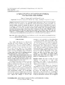
Figure 1.
Cluster Problem for Classification
suits the problem. However, this said, it was however well known that a three layer architecture is sufficient for any classification problem involving many samples which form clusters in feature space(Lippmamm, 1987, see Fig 14 in p.14 and Fig 15 p. 16 in [27]). The idea was that any group of clusters can be separated from the others by confining each cluster inside a polygon (or polytope ) by well defined lines or planes which form the convex hull of each cluster. See figure 2 below.
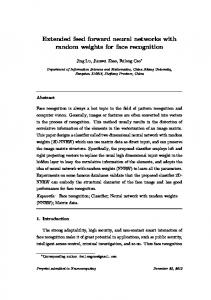
sample points at the boundary of each cluster, leading to the so called Support Vector Machines which was introduced by Cortes and Vapnik [20], but even these could not get over the NP hard problem as was soon realized. (It will be seen later, how by adopting a new approach and the use of the concept of ’Orientation Vectors‘, [29]-[30] the problems of separability and outliers are tackled, see Fig. 4 ). In this paper we describe a method to dodge the problem; we show that it is really not necessary to find the convex hull of each cluster: all we require is that somehow we must be able to separate each cluster from the other by a single plane, if this is done, then the classification problem is much reduced and it can be performed by using a transformation from feature space (X-space) to another S-space in such a manner that each cluster finds itself, after transformation, in an unique quadrant in S-space and thus each cluster is easily classified needing much less planes. See figure 3, where only 4 planes are necessary compared to 43 planes in figure 2.
Figure 3.
Figure 2.
Cluster Problem for Classification solved in conventional way
A classifier can then easily be constructed to discover if any point (sample) lies within any particular polytope (cluster), all the classifier has to do is to check if the particular point lies within the bounding planes which circumscribe the polygon. For example, if the polygon is a triangle, then the classifier can find out if a particular point is within the triangle by verifying that it is within the three sides (planes) of the triangle. If there are many polygons then each of them can be represented by its bounding planes (convex hull), a classifier using ANNs can be built. By this means a three layer ANN network wherein the first layer consists of as many processing elements as the number of planes needed (in figure 2 we need 43) to form the convex hulls of all the polytopes in the sample space[27]. However, this procedure though correct was not practically feasible, and will probably never be, because finding the convex hull of a given region, let alone a number of regions, is a NP hard Problem and especially so in n-dimension feature space where the number of clusters are many and the number of planes involved would exponentially increase. It is appropriate to mention here that around 20 years ago there were attempts to define the convex hull of a cluster by using
Cluster Problem for Classification solved by present method
The purpose of this paper is to show that this can always be done for problems where the clusters are separable, that is if clusters belonging to different classes do not overlap in feature space (of course if there is an over lap there is no method which can work without adding new features in the study - thus essentially enlarging the dimension of the feature space). In very high dimension problems the clusters, in practical cases, will almost always be sparse 2 and this transformation from X-space to S-space performed in such a manner that the codomains are always within one quadrant in S-space is not only feasible but becomes a very powerful tool for classification, actually all the methods and results in this paper has been fashioned from this tool. We introduce the concept of “Orientation” vectors [29]-[30] to keep track of the clusters in feature space and solve the problem. The theorem determines, almost precisely, the number of processing elements which are needed for each layer to arrive at a “minimalistic” architecture which completely solves the classification problem. We further prove that this method of classification is NOT NP hard by showing that if the number of clusters, N, is increased then the number of 2 If there is an image involving 30 x 30 pixels, this means we are dealing with a 900 dimensions feature space, such a space will have 2900 ≈ 10270 quadrants; it will be hard to fill up this space even with one image per quadrant. Thus we see that the sample points are very sparsely distributed in feature space.
3
Figure 4.
Cluster Problem for Classification with outliers
are so devised that the “minimalistic” architecture 3 for each of them is known we can compare the various approximate with the exact solution. This study therefore gives an insight into how one may solve practical problems when the number of clusters are not known and the number of partitioning planes (half spaces) are not known but have to be guessed at. Section 5 is an application section where some suggestions as to how one may “guess” the number of clusters and the number of partitioning planes so that we can arrive at an approximation to the ’minimalistic‘ architecture. In section 6 we show that the present method is not NP hard. We end with a brief discussion on applications on Deep Learning and a Conclusion. 7 is the conclusion. II. A PPROACHES TO THE PROBLEM In this section we will detail our two approaches.
processing elements in this minimalistic architecture, at worst increases linearly with N and at best increases by ∆(log(N )). There are two approaches that can be followed to develop the ideas given in the previous paragraph, but eventually it so turns out that they arrive at the same architecture, these are as follows: (i) We follow Kolmogorov’s approach but give up on the effort of exactly trying to map the exact geometrical domain of the functions, and do not try to obtain a continuous function that maps the exact geometrical domains of each cluster. Instead we use piece wise continuous functions. Further, we only make sure that we can choose planes that can separate one domain (cluster) from another, but assume that on each of these domains a single piece wise constant function is defined. (ii) We give up on the idea of solving the complex hull problem for each cluster (which is NP hard) or even on the idea of trying to confine each cluster within planes (Lippmann 1987) which will form a polygon (or polytope), so that all points that belong to the cluster are inside the polytope. Instead, we just try to look for planes which separate each cluster from another cluster by planes (half space), see figures 1 and 2. We show that if this is done then we can solve the classification problem with much less number of planes figure 3. For the purposes of completeness and also to underline the fact that the ANN method is also a mapping technique and is thus related to the Kolmogorov technique, we describe both methods (i) and (ii) in fair detail in Section 2, though they lead to the same architecture. In section 3, we provide a geometrical constructive proof, that under the conditions put forth in the theorem, which demonstrates how such a three layer network can be had if we are given the details of the piece wise function as described above. This is one of the theorems that we prove. In section 4 we construct example problems wherein we use our methods. These examples have been deliberately constructed with the intent to not only best illustrate the method but also to show how approximations to the classification problem can be made by assuming different ANN architectures and employ the BP algorithm to solve it. Since these examples
A. The Kolmogorov approach As aforesaid, in this paper we solve a more restricted mapping problem which is suitable for most classification tasks. We do not require the general continuous functions of n variables f (x1 , x2 , ..xn ), but only require that our functions be “piece wise constant”, meaning that the functionf (x1 , x2 , ..xn ) take on some constant value in a closed set (region) (ie inside and on the boundary of a particular cluster), therefore the function is continuous for every point of a closed set. For example in figure 3: f (x1 , x2 , ..xn ) can take on some constant value c11 in the region 11 and some other constant value c43 in the region 43 , etc. in fact there is no loss of generality if we assume that c11 equals the class number 1 of the particular cluster 11 ie we may define c11 = 1, similarly we may define c43 = 3, 3 being the class number of cluster 43 . We further assume that the domain of each function is separable from other domains by planes (ie they are separable). This assumption allows us to immediately exploit the idea of finding the minimal number of planes that can separate the domains, thus if we know how a point (belonging to a domain) is “oriented” with respect to all the planes then we can quickly find out as to which domain the point belongs to. To draw a parallel with the work of Kolmogrov, we have found a way to map a “piece wise constant” function defined in n-dimension space to a function defined in discrete 1dimension space. A “piece wise constant”’ function in ndimension space f (x1 , x2 , ..xn ) (which takes input as points in the n-dimensional feature space and outputs the class number of that point) is mapped to an equivalent 1-dimensional function (v(u)) which takes input as the cluster number to which the point in n-dimensional feature space belongs and outputs the corresponding class number. The function (v(u)) takes as input one among a discrete set of values (cluster number) and its set of all output values also forms a discrete 3 The term ‘minimalistic’ that we use should be interpreted with caution, it generally means an architecture with the minimal number of processing elements in the 1st layer, this too is a bit imprecise: what we mean is the number of layers when we use a sigmoid function si = tanh(βyi ) with β large, say, β > 5. With smaller values of β it is possible to arrive at an architecture which has a few processing elements less than the this ‘minimalistic’ value, a point which becomes clear later on.
4
set (class number). Our construction also shows a unique way to map points in the n-dimensional feature space to their corresponding cluster number. By this method we use planes S1 ,S2 , S3 to separate the domains and perform the mapping. We will see that these planes are the same planes that are used in the second approach (next subsection), to separate the clusters in such a manner that no two clusters are in the same side of all the planes. B. Orientation Vector approach In this approach we use the concept of an ‘orientation vector’ to provide a geometrical constructive proof, under the conditions put forth in the theorem, which demonstrates how such a three layer network can be had if we are given the details of the piece wise function as described above. The proof also provides a method which would overcome some of the difficulties in arriving at a suitable architecture for a given data in a classification problem. It is shown that given a data set of clusters in feature space there exists an artificial neural network architecture which can classify the data with near 100 percent accuracy (provided the data is consistent and the train samples describe a convex hull of each cluster). Further, it is shown how by using the concept of an “orientation vector” for each cluster, an optimal architecture is arrived at. It is also shown that the weights of the second hidden layers are related to the orientation vector thus making the classification easily possible. We give 3 examples on the method each of increasing complexity. The purpose of these examples is to show how once the architecture of the network is fixed, the weights of the network can be easily obtained by using the Back Propagation algorithm to a feed forward network. III. S TATEMENT OF T HEOREM AND P ROOF Suppose there are m clusters of points in n dimensional feature space, figure 5 is a typical depiction, such that each cluster of points belongs to one of k distinct classes, and further if there exist q distinct n−dimensional planes which separate each cluster from its neighbors in such a manner that no two clusters are “on the same side” of all the planes, then it is possible to classify all the clusters by means of a feed forward neural network consisting of three hidden layers which has an architecture indicated as: q − m − k. That is the the neural network will have q processing elements in the first hidden layer, m processing elements in the second layer, and k processing elements in the last layer. The input to this neural net work will be n−dimensional, that is it will be the coordinates of a data point in n−dimensional space whose membership to a particular class will be ascertained uniquely by this neural network. The out put of this network will be k binary numbers, out of which only one of them will be 1 and the rest will be zero. In the k-dimensional output vector if the the first component is 1 then it means the input vector belongs to the first class, or if the second component is 1 it means that the input vector belongs to the second class ....and so on to the last (kth class ). In some notations which include
Figure 5.
Cluster of sample points in n-dimensional space
the number of inputs, then the architecture would be denoted as: n − q − m − k. In the figure 5, we have chosen: q=5, m=8 and k=3, there are 8 clusters number 1 to 8, the suffix indicates the class assignment, for example cluster number 4 is denoted with a suffix 3 ie as 43 this just indicates that the points in this cluster belong to class 3, it may be noticed that there are other points in cluster number 8 which also belong to class 3. NOTE A: It is assumed that the q planes do not intersect any cluster dividing it into two parts, if there happens to be a particular cluster which is so divided i.e. if there is a plane which cuts a particular cluster into two contiguous parts, then the part which is on one side of this plane will be counted as a different cluster from the one which is on the other side : that is the number of clusters will be nominally increased by one : m to m + 1. NOTE B: It may be noticed that we assume that all points in a cluster belong to a single class (though the same class may be spread to many clusters, this assumption is necessary else it means that the n-features are not enough to separate the classes and one would require more features. Example suppose there is a sample point R which actually belongs to class 2 inside the cluster 43 , this means class 2 and class 3 are indistinguishable in our n-dimensional feature space and there should be more features added, thus increasing n. The proof of the theorem of course assumes that the dimension, n, of the selected feature space is sufficient to distinguish all the k classes. NOTE C: Perhaps it is superfluous to caution that figure 5 is a pictorial representation of n-dimensional space and a plane which is merely indicated as a single line is actually of n-1 dimensions and the arrow representing the normal (out of the plane) is perpendicular to all these n-1 dimensions. We prove our theorem by explicit construction. To fix our notation we have provided a diagram which shows the architecture of a typical neural network shown in the figure 6, whose architecture is chosen for classifying the clusters given in figure 5. However before proceeding to the proof we need a few definitions: We first define what is meant by the terms “positive side” and “negative side” of a plane. We indicate by an arrow the normal direction of each plane S1 , S2 , ...Sq (in the figure we
5
we have similar formulae for all the processing elements, Sj , j = 1, 2, ...q in the first layer, the last q th being: sq = tanh(βyq ) where yq = wq0 + wq1 x1 + wq2 x2 + .... + wqn xn
Figure 6.
Neural network architecture proposed in this paper
have taken q = 5). It may be noticed from figure 5 that all the points in the particular cluster indicated by 11 is on the side of the arrow direction of plane S1 , hence we say that 11 lies on the “positive side” of plane S1 ,or as “+ve side” of plane S1 , points on the other side of this plane is defined to lie on the “negative side” of plane S1 or as “-ve side”. So we see each cluster will be either on the positive side or on the negative side of each plane, because by assumption no plane cuts through a cluster, (See Note A). Now we define a “orientation vector” of a cluster as follows: Let us take the cluster indicated by 11 we see that this cluster is on the +ve side of S1 , +ve side of S2 , -ve side of S3 , +ve side of S4 and +ve side of S5 , this situation is indicated by the array (1, 1, −1, 1, 1). We thus introduce the concept of a orientation vector of the cluster 11 as a vector which has q components and is defined as d(11 ) = (1, 1, −1, 1, 1). To take another example, let us take the cluster 43 its orientation vector is d(43 ) = (−1, −1, −1, 1, 1) as can be ascertained from the figure. So we can, in general denote the orientation vector of any cluster b as db = (db1 , db2 , ...dbr , ..dbq ); where dbr = +1 or -1 according as cluster b is on the +ve or -ve side resp. of plane r. It should be noted that the orientation vector of each cluster is unique and will not be exactly equal to the orientation vector of another cluster; this will always happen if the orientation vectors for each cluster are properly defined. Thus the dot product db .dc of the orientation vectors vectors of two different clusters b and c will always be less than q: db .dc = q , if b = c and db .dc < q , if b 6= c actually it is because of the above property and the uniqueness of each orientation vector, that we are able to build the architecture for any given problem. The out put of the first processing element in the first layer denoted by S1 in the figure is: s1 = tanh(y1 ) s1 = tanh(βy1 ) where we arbitrarily choose β = 5 y1 = w10 + w11 x1 + w12 x2 + .... + w1n xn it may be noted that the formula w10 + w11 x1 + w12 x2 + .... + w1n xn = 0 corresponds to the equation of the plane S1 of figure 6.
where wq0 + wq1 x1 + wq2 x2 + .... + wqn xn = 0 is the equation to the plane Sq of figure 6. Since the planes S1 , S2 , ..Sq are assumed to be given, the coefficients (weights) wij of all the processing elements in the first layer are all known. NOTE D: Now we wish to make a very important observation, which has a bearing on the many things that we will be dealing with. It may be noticed that the immediate out put of the first layer viz (y1 , y2 , .., yq ) passes through the sigmoid functions tanh(βyi ) (with β large, say, β = 5)and then produces a vector (s1 , s2 , .., sq ). But since the sigmoid function si = tanh(βyi ) maps almost all the points yi (which are bit far away from yi = 0) to a point close to either si = −1 or si = +1, we see that as a consequence that every input sample (x1 , y2 , .., xn ) maps to (s1 , s2 , .., sq ) where (s1 ≈ ±1, s2 ≈ ±1, .., si ≈ ±1, .., sq ≈ ±1) that is the image point in S-space is always close to some q-dimensional Hamming vector which is (±1, ±1, .., ±1) . Definition of the “Center” of a Quadrant in S-space: Suppose a point Q has a coordinates which can be expressed as a Hamming Vector say (1, −1, 1, .., 1), then we consider Q as the “Center” of that quadrant of the space whose points are having coordinates: (s1 > 0, s2 < 0, s3 > 0, .., sq > 0). Eg (i) The point Q’ whose coordinates are (1, 1, .., 1) is the “Center” of the “first” quadrant whose points are having coordinates: (s1 > 0, s2 > 0, s3 > 0, .., sq > 0), similarly Eg. (ii)the point Q” whose coordinates are: (−1, −1, −1, .., −1) is the “Center” of the last” quadrant whose points are having coordinates: (s1 < 0, s2 < 0, s3 < 0, .., sq < 0) . since, we are in qdimensional space there are 2q quadrants, this provides an upper limit to the number of clusters that can be separated by q planes viz. 2q . So a worthwhile observation to make is that the images of all the points which are not near any dividing plane Si will be points close the Center of some quadrant in S -space. Further, all points belonging to a particular cluster get mapped to a region very close to the center of a particular quadrant, in other words all the images of one particular cluster will be found near the center of its own quadrant in S-space. (We will see later that this last property makes it easy to employ a further mapping if we wish). Since all points belonging to a single cluster gets mapped to its unique quadrant in S-space, (uniqueness certainly follows because of the uniqueness of each orientation vector, that is when the planes are well chosen) and the we can easily classify them by “collecting” the points in each quadrant. This is done by writing down the appropriate weights of the processing elements in the second layer, which we call the “Collection Layer”, because of its function. Let us start with the first one which is shown as 11 in the figure 6.
6
The output u1 = tanh(βz1 ) where 0 0 0 0 z1 = w10 + w11 s1 + w12 s2 + .... + w1q sq
Now since we wish the the first processing element to output u1 = +1 if the input n-dimensional vector x1 , x2 , ..., xn belongs to the cluster 11 and to out put u1 = −1 if it belongs to any other cluster, we see that this condition will be adequately satisfied if we choose: 0 0 0 0 (w11 , w12 , w13 , ..., w1q ) = (d111 , d121 , d131 , .., d1q 1 )
which we write in short hand as: w0 1 = d11 0 and the constant term: w10 = 12 − q . It can be easily seen that if the sample point x1 , x2 , ..., xn belongs to the cluster 11 then z1 = 1/2 and hence the out put u1 = tanh(βz1 ) becomes very close to +1, else the out put becomes very close to -1. Similarly the second processing element indicated as 22 will output u2 = tanh(βz2 ) where 0 0 0 0 z2 = w20 + w21 s1 + w22 s2 + .... + w2q sq
and if we choose 0 0 0 0 (w21 , w22 , w23 , ..., w2q ) = (d212 , d222 , d232 , .., d2q 2 )
ie. w0 2 = d22 0 and the constant term: w20 = 12 − q We can now write down the general term viz the output of the ith processing element belonging to the jth class: ui = tanh(βzi ) where 0 0 0 0 zi = wi0 + wi1 s1 + wi2 s2 + .... + wiq sq
and if we choose i
i
i
0 0 0 0 (wi1 , wi2 , wi3 , ..., wiq ) = (d1j , d2j , d3j , .., diqj )
ie. w0 i = dij 0 and the constant term: wi0 = 12 − q It can be easily seen that if the sample point x1 , x2 , ..., xn belongs to the cluster ij then zi = 1/2.
This is easy to do, we choose the connection weight between the processing element in the second layer say ij and processing element l of the last layer as equal to the Kronecker delta δjl ;(by definition δjl = 1,if j = l else δjl = 0 ). Thus we explicitly write vl = pl0 + pl1 u1 + pl2 u2 + .. + pli ui + .. + plm um where we now define pl0 = 0 and we choose pli = 1 if the cluster ij belongs to class l, that is j = l, else we define pli = 0 With the above choices all the weights in the network are now known, thus completely defining the Neural Network which can classify all the data. To demonstrate why it works let us consider, in figure 6,the connection weight between the processing element 11 and the processing element 1 (in the last layer)p11 = 1, but the connection weight to 2 p21 = 0. Similarly, the connection weight between the processing element indicated as 62 and 1 p16 = 0, the connection weight between 62 and 2, p26 = 1 and the connection weight between 62 and 3, p36 = 0; thus ensuring that if the input point (x1 , x2 , .., xn ) belongs to the cluster 62 then it will be classified as class 2. We thus see that the neural network will out put a point belonging to a cluster ij to the class j as required, since the jth processing element outputs vj a number which is equal to 1 as the final output; the other vk , k 6= j will out put 0. QED. B. Four layer problem We have seen that the out put of the first layer maps all points onto S-space; and since each cluster is mapped to its “own quadrant” in this space the problem has already become separable. It was only necessary to identify the particular quadrant that a sample had got mapped to, in order that it can be classified; a task undertaken by the collection layer. Though the above section shows that the number of layers (three) is sufficient, it is sometime better to make one more transformation from the S space to h space by using orientation vectors in this space (see figure 7) this could lead to a network with with less processing elements in the layer.
A. Use of Unit Step Function Now to simplify the proof we will use the Unit Step Function instead of the activation tanh function in the second layer, ie. instead of defining ui = tanh(βzi ) as above, we use the unit step function U sf (z), which we define as:U sf (z) = 1 if z > 0 else U sf (z) = 0. The output ui = U sf (βzi ) becomes 1 or 0 (binary). This we do only to demonstrate the proof, but in actuality in practical cases the original tanh function would suffice with some appropriate changes in the equations below. Now we come to the last layer:
Figure 7.
Cluster within a cone
7
(That is if there are clusters belonging to the same class in one half space then it is not necessary to separate these clusters individually since anyway they belong to the same class, we can save on the number of planes if we group such clusters as belonging to a single region.) The figures, show how such regions, containing “clusters of clusters” belonging to the same class can be separated by planes. In this section we show how all this can be done by introducing another layer before the “Collection Layer”. Also the Collection Layer in this case collects samples belonging to one region which has samples belonging to possibly more than one cluster but all belonging to the same class. This becomes apparent in the figures which depict the orientation vectors H, in the s-space.
Figure 8.
Clusters in conical pencils
The above diagram shows that there are several places where clusters belonging to the same class can be grouped as one region containing a“cluster of clusters”, these regions can then be separated by fewer planes (the figure 8 shows 4 planes and to prevent clutter the cone containing Region 222 in the negative side of H1 and separated by the positive side of H2 has not been drawn). The Architecture for such a situation can be easily arrived at by introducing the orientation vectors H as another layer . We than have the architecture shown in figure 9.
Figure 9.
IV. EXAMPLES We now, for the purpose of illustration, solve a few problems and show that for a given classification problem if a neural network architecture is chosen as per the above theorem then the classification is guaranteed to be 100% correct, provided the data satisfies all the conditions of the theorem. A NOTE On Choice of Examples: These examples , were purposely constructed because we need to know exactly the geometrical configuration of each cluster and the number of points involved and how the clusters are nested one within an another. So even though the example may seem artificial and the first one seems to be a "toy" example, they were purposely constructed so that we can theoretically calculate the minimum number of planes require to separate the clusters. This latter information is very important to us otherwise there is no way of comparing our results with the "exact" result. However, the examples become increasingly complex in Sec IV E we have r-levels of nested clusters one within another in n-dimensions, and yet they are so constructed that we know the number of planes that will separate them! First the 3 layer architecture is chosen as per the configuration dictated by the theorem, then the Back Propagation algorithm is used to show that in each of the 3 example problems the classification is 100%. Secondly, we introduce a fourth layer; since we cannot know the number of processing elements in the second and third layers, different configurations were tried. This is just to show that even if we do not know the exact number of clusters we can by a judicious guesses choose processing elements in the second and third layer in such a manner that the classification is done 100% or near 100%. The 3 Examples (below) are constructed in such a way that we know the number of clusters, the number of classes and also which cluster belongs to which class. For convenience we assume the shape of all the clusters, in the examples, to be spherical. In all the examples we generate the coordinates of sample points within clusters and coordinates of test points by using random number generators. We then use the backpropagation method after choosing the appropriate architecture as dictated by the above theorem for the 3 layer case and a variety of architectures for the 4 layer case. (Later, in sections V(B) and V(D), we give techniques of choosing a suitable architecture). The 3 examples are: (A) The 3D cube, (B) The 4D cube and (C) The 4D nested cubes. We then generalize in para (D) the nested cubes to n dimensions and in para (E) consider r levels of nestings in n-dimensions and give a minimalistic architecture for these and draw interesting comparisons with Radial Basis Function classifiers. TEST RESULTS ON EXAMPLES:
Neural network architecture of a four layer network
A. Three Dimensional Cube In the example problems below, we did not use the Unit Step function but rather used the Tanh function to enable the use of Back propagation algorithm ([16]). So the outputs will be in the range [−1, +1], and all positive points are treated as +1 and all the negative points are treated as 0.
This is a 3-d problem involving a cube which is centered at origin and whose neighboring vertices at a distance of 2 apart from each other. There are 8 clusters, centered at each of the vertices, we assume that each cluster has a radius of 0.3. The symmetrically opposite vertices of the cube belong to the same class, and hence there are a total of 4 classes. For
8
example, the symmetrically opposite vertex of (1, -1, 1) is (-1, 1, -1). We use the same definition of symmetrically opposite vertices in the remaining examples in this paper. For instance, in example IV-B, the symmetrically opposite vertex of (-1, 1, -1, 1) is (1, -1, 1, -1). Therefore the points belonging to the clusters around these vertices belong to the same class. We have drawn samples from these clusters to formulate the train data set, these are 100 sample points randomly generated within each spherical cluster (100 samples per cluster) and test data set (50 samples per cluster). A feed-forward neural network was then trained to classify the training data set. The architecture of the network is as follows: dimension of the input layer is 3, dimension of the first hidden layer is 8 (equals the assumed number of planes required to split the clusters, though for this simple case the 3 coordinate planes are sufficient to split the clusters we do not use this information),dimension of the second hidden layer is 8 (equals the number of clusters) and the dimension of the output layer is 4 (equals the number of classes). Therefore by using the network architecture: 3-8-8-4 The feed forward neural network was trained using Back propagation algorithm and it gave 100% classification accuracy on both the training and test data sets. B. Four Dimensional Cube This is a 4-d problem involving a hypercube which is centered at the origin and whose neighboring vertices at a distance of 2 apart from each other. For convenience we assume the shape of the clusters in this and the next problem to be that of a 4d sphere. There are thus 16 spherical clusters, centered at each of the vertices, and having a radius of 0.3. The symmetrically opposite clusters of the 4-d cube belong to the same class, (i.e. if the cluster centered at the coordinate (1,1,1,1) belongs to class 1, then the cluster whose center is situated at (-1,-1,-1,-1) also belongs to class 1. Hence, there are a total of 8 classes. As in the above experiment, we have drawn samples from these clusters to formulate the train data set (100 samples per cluster) and test data set (50 samples per cluster). A feed-forward neural network was then trained to classify the training data set. (i) Using the 3 layers of processing elements in the architecture: The architecture of the network is as follows: dimension of the input layer is 4, dimension of the first hidden layer is 16 (equals the assumed number of planes required to split the clusters), dimension of the second hidden layer is 16 (equals the number of clusters) and the dimension of the output layer is 8 (equals the number of classes). (a) Using: 4-16-16-8 architecture, the Back propagation algorithm produced 100% classification accuracy on both the training and test data sets. (b) Actually for this problem we can show that just 4 planes are sufficient to separate the cluster, these are the 4 coordinate planes: x= 0; y=0; z=0; t=0; ii) Using the 4 layers of processing elements in the architecture: (a) 4-16-2-8
(b) 4-15-5-8 (c) 4-9-9-8 The feed forward neural network was trained using Back propagation algorithm and it gave 100% classification accuracy on both the training and test data sets. C. Nested Four Dimensional Cubes Here we consider a 4-d problem of a big hypercube which has smaller hypercubes centered at each of its 16 vertices. That is each smaller hypercube has its center at one of the vertices of the larger hypercube. Thus a total of 256 spherical clusters belonging to 8 classes. The neighboring vertices of the bigger hypercube are at a distance of 4 apart from each other. The vertices of this bigger 4-d cube form the center of the smaller 4-d cube. The neighboring vertices of the smaller hypercube are at a distance of 2 apart from each other. Hence there are 256 (16x16) clusters having a radius of 0.7 (there are no clusters at the vertices of the bigger hypercube) Now we classify each cluster as follows. As in the example IV-B, each small hypercube will have 16 clusters and clusters symmetrically opposite will belong to the same class, thus there are 8 classes for each small hypercube. As there are 16 small hypercubes there will be 256 clusters belonging to 8 classes. Note we have imposed a symmetry to our problem by placing all the cubes in such a manner that the edges of each of the cubes are parallel to one of the coordinate axis. This symmetry has been imposed on this and all the subsequent examples considered in this paper. (i) Three layer of Processing elements: As in the above experiment, we have drawn samples from these clusters to formulate the train data set (100 samples per cluster) and test data set (50 samples per cluster). A feed-forward neural network was then trained to classify the training data set. The architecture of the network is as follows: dimension of the input layer is 4, dimension of the first hidden layer is 256 (equals the number of planes, which was purposely chosen very high and equal to the number of clusters), dimension of the second hidden layer is 256 (equals the number of clusters) and the dimension of the output layer is 8 (equals the number of classes). Thus the architectures tried out is: (a) 4-256-2568, The feed forward neural network was trained using BP algorithm, which converged in less than 500 epochs, and it gave 100% classification accuracy on both the training and test data sets.We have chosen the number of planes as 256 (equal to the number of clusters), which is sufficient to distinguish all the clusters from one another by a 256 dimension orientation vector. Actually, it would not have mattered even if we had chosen more planes than 256. However, it may be noticed that because of the symmetry of the configuration, only 12 planes are actually required to separate all 256 clusters, these planes are: x= 0; y=0; z=0; t=0; x= 1; y=1; z=1; t=1; x= -1; y= -1; z= -1; t= -1; so an architecture of the type 4-12-256-8 is theoretically sufficient for this problem, therefore by using various architectures we got results as per this table: (a) 4-12-256-8 : 99.852% train & 99.672% test (b) 4-13-256-8: 99.191% train & 99.117% test (c) 4-14-256-8: 99.891% train & 99.641% test
9
(d) 4-18-256-8 :100% train & 99.969% test (ii) Architectures with Four layers of Processing elements which also worked are: (e) 4-12-40-300-8 (f) 4-12-100-150-8 (g) 4-12-120-80-8 (h) 4-12-50-50-8 D. Generalization of Nested Cube Problem to n dimensions The problem 3 which has clusters of smaller cubes placed at corners of larger cubes can be generalized to n− dimensions. There will be a large n-dimension cube with smaller ndimensional cubes at the corners: so we have 22n clusters and if each pair of “diagonally opposite” clusters in the smaller cube belong to the same class then there will be 2n−1 classes. We require only 3n planes to separate the clusters so the minimal neural network architecture will be : n − 3n − 22n − 2n−1 . This problem is interesting because a Radial Basis Function method would involve 22n distance measurements to classify a single sample, where as by this method there are only 3n linear equations to be evaluated to obtain the unique Hamming vector which identifies the same sample. E. Generalization to sequence of nested cubes one inside the other In fact we can still further generalize the n dimensional example given in the previous section. Suppose we define the previous example as level-2 nesting: that is we take a large n-dimensional cube and place smaller n-dimensional cubes at the vertices, each of these small cubes have a cluster at its vertex. Now we can consider such level-2 structures placed at the vertices of a still larger n-dimensional cube we get a level3 structure (ie level-2 nested cubes at the vertices of another large cube). So we can go on to get a level-r nested structure. This level-r nested structure will have 2rn clusters belonging to 2n−1 classes. It can be shown that such a cluster can be distinguished by using (2r − 1)n planes and thus we will have a NN architecture: n − (2r − 1)n − 2rn − 2n−1 . There are only (2r − 1)n linear equations to be evaluated to obtain the unique Hamming vector which identifies a sample which may belong to any one of the 2rn clusters and finds which of the 2n−1 classes it belongs to. These (2r −1)n linear evaluations may be once again compared with 2rn distance measurements which would be necessary, to classify a single sample, if one uses the Radial Basis Function method. V. A PPLICATION TO C LASSIFICATION P ROBLEMS Now it is probably appropriate to answer the query: What type of patterns and what type of cluster configurations can be easily classified by our method? It would be quite apparent by now that if the patterns are in clear clusters like those given in Example 1 and 2 (Level 1)then the problem is completely classifiable by using the above mentioned neural architecture, the EXAMPLES section clearly illustrate this (in particular problem 1 and 2, viz the 3-d and 4-d cubes). However in some other cases wherein we have clusters within clusters, Level 2, (eg. problem 3; the nested 4-d cube); that is when each large cluster contains sub-clusters, much like a cluster
of galaxies each of which is a cluster of stars, some more investigation needs to be done. For these and other cases (cluster configurations of Level-r), it is possible to estimate the number of planes required. However, the precise number of planes would depend on the number of clusters and their geometrical positions in feature space. So we can only make an estimate. This estimate helps determine a possible architecture for the Neural network classifier.Before proceeding to our estimates, we would first need a definition. Malleable cluster: We will define (consider) a cluster as ’malleable’ if (i) a sample point is classifiable to a cluster by just taking its Euclidean distance to the centroid of a cluster, OR (ii) a sample point can be associated to its cluster by a k nearest neighbor algorithm. All clusters will be assumed to be malleable. We further assume that different clusters are separable from one another by planes, if necessary a cluster may be divided into two or more parts to facilitate such a separation (see figure 4). We wish to say without being ad nausea that in cases where clusters belonging to different classes overlap with each other then it is not possible to classify the problem without using probabilistic techniques and we do not consider such situations in the paper. It could also mean that we have not taken enough number of relevant features to solve the problem. ESTIMATION OF NUMBER OF PLANES In the next three subsections, we give methods with heuristic proofs on how to estimate the number planes which can separate Level 1 and Level 2 clusters and also for the case when the clusters are not too sparse. Though our proofs are heuristic, it may be mentioned that our estimates are in concordance with the bounds proved by Ralph P. Boland and Jorge Urrutia [28],1995, who in their work had elegantly exploited the crucial fact: In n-dimension space a single plane, in general, can simultaneously separate n pairs of points(randomly placed, but not all in the same plane), thus if we choose the first pair of 2n points (among N), the first plane thus cuts these 2n points and places them into two sets one on either side of the plane,4 this plane of course divides the other points among N to to either side; after this n new pairs of 2n points are chosen such that each pair is unseparated, a second plane is then chosen which divides the new n pairs and also the space to 4 ’quadrants’ , the next plane gives 8 ‘quadrants‘, the process continues and new planes are added, but must quickly end because all the N points will be soon exhausted.5 The proofs by Boland and Urrutia[28]are involved though rigorous.
4 Another way of looking at this is to think that each pair of points as a line segment which has a midpoint, since there are n pairs, one can always find the n coefficients αi , (i = 1, 2, .., n) of a plane (say) 1 + α1 x1 + α2 x2 + .. + αn xn = 0 which passes through these n midpoints. 5 Another crucial point to note regarding n-dimensional geometry: Every time you add a plane in n-dimensional space you are dividing the space and doubling the number of existing number of ‘quadrants’, but this doubling happens only for the first n planes the (n + 1)th plane will not double the ‘quadrants’ but create a ‘region’ confined by other n planes. Remember we have chosen n large and N < 2n .
10
A. Estimate of number of planes: Clusters of Level 1
We show that for problems, involving large n-dimensional feature space, which has N clusters, N < 2n , sparsely and randomly distributed and configured as Level 1, the number of planes q are O(log2 (N )). As is known a 2d space has 4 quadrants,3d space has 4 quadrants and n dimensional space has 2n quadrants. Suppose the dimension of the feature space is large (say 40), then it is most likely, in practical situations such as face recognition, disease classification etc., that the number of clusters (say 10000), will be far less than the number of quadrants, (as 240 ≈ 1012 ) that is, the number of clusters will be sparsely and randomly distributed. Therefore an interesting question arises: Is it possible to transform the feature space X of n-dimension to another n-dimensional Z space such that each cluster in X space finds itself to be in one quadrant in Z space, such that each cluster is in a different coordinate in this Z space? If this is so then the problem can be tackled in Z space instead of the original feature space, thus making the classification problem trivial. The answer to the question is yes, if the cluster configuration is of type Level-1 In fact, the present problem is closely related to the problem first dealt with by Johnson and Lindenstrauss [21](1984), who showed that if one is given N points in a large n dimensional space then it is possible to map these N points to a lower dimension space k of order k = log2 (N ), in such a manner, that the pairwise distances between these points are approximately preserved, (in fact our requirement is much less stringent we only require that the ‘centroid’ of N clusters, be mapped to a different ‘quadrant’). The transformation is easy: Every point P, in n dimension space, whose coordinate is xP and which belongs to cluster i can be transformed to x0 P another point in n dimension space. This transformation from X space to X 0 space is given by : x0 P = C i +(xP - xi ) Where xi is the centroid of cluster i in the X space; C i is the coordinate of the point to which the centroid of i has been shifted in X 0 space. We can choose C i to be sufficiently far away from the origin such that its distance, from the origin of X 0 space is larger than the radius of the largest cluster (for convenience, we can choose the origin of the X 0 space to be the global centroid of the sample space). Typically, if n = 5 we could choose some point say, C i = D(1, 1, −1, 1, −1) where D is sufficiently large. Thus we see that the problem is classifiable in X 0 space, and a classifier with (say) q planes, q = log2 (N ), exists and since the transformation from X space to X 0 space is essentially linear and the clusters are sparse in X 0 space and can be separated by these q planes, then a similar classifier exists in x space. In X 0 space the centroid of each cluster can be given ‘coordinates’ by measuring the perpendicular distance from each of the q planes to get the ‘coordinates’ (z1, z2, ...zq), ie related to the orientation vector, therefore each cluster will be in a ‘quadrant’ of the q dimensional z space. A situation somewhat similar to Johnson and Lindenstrauss [21]-
[22] because q = O(log2 (N )). QED.6 From the above we see that problems involving labeled data in class 1 are always classifiable by transformation into Z space. Thus we see when the number of clusters N are such that N < 2n , n being the dimension of space, then we require only q planes q = log2 (N ). In the example we see that Problem 1 and Problem 2 are problems of class 1 type. further, problem 1 is a cluster in three dimension space involving 8 clusters in this case 8 is equal to 23 , hence we see that the clusters are sparse and hence it can be solved by using only 3 planes the equations of these 3 planes are x=0, y=0, and z=0. Similarly in Problem 2 we have a 4 dimension cube involving 16 clusters which is equal to 24 , here again we need only 4 planes whose equations are x=0,y=0,z=0 and t=0. In problem 3 we have too many clusters (256) which is much more than 24 . Therefore, we will deal with this case later. B. Estimate of number of planes: Clusters of Level 2 Here again we assume that the number of clusters N, N < 2n . In this case, there is a large cluster involving ’regions‘ each of which consists of clusters (analogous to galaxies and stars). We can solve this as follows: we divide the problem into K regions such that each region does not have more than 2n clusters. We can separate these K regions by log2 (K) planes and each of these have a max of N’ ≈ N/K clusters in a region by log2 (N 0 ) planes, thus the total number of planes q, would be O(Klog2 (N/K)) + O(log2 (K)). We can estimate the number of planes by repeatedly using the logic of the previous paragraph for clusters of Level-r. In problem 3 we have too many clusters (256) which is much more than 24 . These are 16 large clusters each containing 16 smaller clusters therefore one would have thought that they would require 16 X 4 + 4 =68 planes, however from the symmetry of the problem we see that we require only 12 planes. Therefore we see that 3, 4, and 12 planes are sufficient to solve problems 1, 2 and 3 respectively; these are the minimal. Now it is interesting to see if the BackPropagation algorithm can discover the weights of the planes if the number of planes are specified, we report that if the cluster sizes are small and if the separation between clusters is large than the algorithm succeeds, else more number of planes are required. Details are provided in the Example section. What happens if we have labeled clusters and if we do not know the number of clusters? We have seen (in the Example section) that we need to approximately guess the number of clusters as m and if the problem is of Level-1 than choose the number of planes to be a little higher than log2 (m). In fact if we choose the number of planes is equal to the number of clusters, the upper limit, the problem is automatically resolved but this is inefficient. In the Example problems, we did start 6 An alternative argument can be had by transforming all the points in Xspace of n dimension to points on the surface of a sphere (radius R) of n+1 dimensional X’-space. After, choosing the origin as the global centroid of all the clusters, we use the transformation x0i = Rxi /A (i = 1, 2, .., n); and x0n+1 = R/A with the choice A = (1 + x21 + x22 + ..x2n )1/2 . The clusters on the sphere can be separated from one another (because they are sparse) by (say) q ‘great circles’, each contained in a plane through the origin. We thus arrive at the same result.
11
with this rather inefficient guess (by assuming the number of planes as equal to the number of clusters) and apply the BP algorithm. We then solved the examples by using a variety of more efficient architectures which were then trained by the Back Propagation algorithm.
Architecture 4-12-256-8 4-13-256-8 4-14-256-8 4-18-256-8 4-256-256-8
Train Accuracy 99.852% 99.191% 99.891% 100% 100%
Test Accuracy 99.672% 99.117% 99.641% 99.969% 100%
KCR 18.81 17.95 17.16 14.52 1.48
PEW 18.74 17.79 17.10 14.51 1.48
C. Problems when the number of clusters are not sparse We had assumed that the number of clusters are sparse. What happens if the number of clusters are not smaller than 2n ? In this case we use the method previously try to divide the total number of clusters as belonging to different regions. Choose K regions, such that each of the K regions does not have more than 2n clusters. Of course the final answer will depend on the geometrical distribution of the clusters. See ref [28] for further details on this subject. D. Some points for implementation in practical classification problems For the sake of completeness, we briefly suggest a means of implementation of the method of classification described in this paper for practical cases. (i) Choosing an Architecture The procedure for software implementation could be as follows: When data is first given, a suitable nearest neighbor clustering algorithm may be applied (may be done after suitable dimension reduction). This will give the number of clusters as shown in figure 5. The number of separating planes will be ascertained or estimated. Normally for sparsely distributed, N, clusters in high n-dimensional space, the number of planes will be O(log2 (N ), in practical cases the number of planes can be taken to be 30% or 40% more than log2 (N ), the exact number of planes are not necessary because an over specification does not matter, the number of layers of processing elements will be three, thus the architecture of the ANN is known as the number of classes is known for a supervised problem. Then the well-known back propagation (BP) algorithm could be employed using this chosen architecture to solve the classification problem just as what was demonstrated in section IV. (ii) Evaluating a chosen Architecture Suppose we have two Architectures, which give equally good predictions,how do we say which is better? One way is to use the concept of Occum’s Razor, in order to do this we could use the following two ratios: (i) the ratio of the ‘number of equations’7 fitted (while training) to the total number of weights used in the neural architecture, we may call this the knowledge content ratio per weight (KCR),(ii) the second ratio is nothing but the first multiplied by the fraction of correct predictions (fcp)on unseen test samples, this would give the prediction efficiency per unit weight (PEW), P EW = KCR.f cp It is best to use that architecture which has the highest possible KCR or PEW. The Table shown above gives the values of KCR and PEW for problem 3 (the nested 4 d clusters), for a variety of architectures which were trained using BP. 7 We define the ‘number of equations’ as the total number of conditions imposed while training.This is equal to number of training samples multiplied by the number of processing elements in the last layer.
VI. T HE METHOD OF ORIENTATION VECTORS IN NOT NP HARD
Suppose we have arrived at our so called “Minimalistic” architecture by using the method of Orientation vectors for solving a particular problem involving N clusters and k classes. (It is assumed that in this section we are dealing with large dimension space with sparse cluster). Now what happens if we increase the number of clusters by ∆(N ) and the number of classes from k to k+1? By this time, we have covered enough ground to be able to answer this question. Suppose we a have a certain number of clusters say N = Nf , in a large n dimension space, how do we begin to separate them by planes? We will now describe such a process. We start with a certain number of clusters in an initial set (say) N = N0 , belonging to the actual configuration of N = Nf clusters and then choose an initial set of planes q = q0 , to separate these N0 , as a start 8 we will assume N0 i > m < j < l < n . The variables (y1, y2, .., ym ) can be considered as the reduced “independent” variables 11 and the input data as n-dimensional dependent variables in x space.
Figure 11.
A Typical Configuration of an Auto encoder (MNN)
The purpose of this section is just to demonstrate only two facts: (i) That the mapping performed by a fully trained auto encoder (MNN) is such that each cluster starting from a cluster 11 Think of a sample vector (point) in X space as a large sized photograph involving n pixels and its reduced sized photograph of m pixels as a vector in Y space representing the same photograph, m < n, in addition we may have to think of m as a measure of the smallest sized photograph (the smallest number m), which can be used to distinguish the photographs in the input set one from another.
in an input layer is mapped to a unique cluster in the next layer,and this is true from layer to layer. To prove this we take a simpler MNN shown below:
Figure 12.
A Simple Auto encoder (MNN)
The mappings made by the above architecture are shown pictorially below:
Figure 13.
Mapping Property of Auto encoder (MNN)
It is clear that since we want the MNN to “mirror” each vector this property of the mapping moving from one cluster to another is correctly depicted for points 1 and 2 as shown above. The case of points 3 and 4 which start from different clusters and land in the same cluster cannot happen, because if the points 3 and 4 land up in the same cluster (as shown for e.g. in Y-space), the network cannot “mirror” the input thus the input vector cannot be recovered. This property is important because it leads to an important Theorem which shows that such MNN architectures can be used for hierarchical classifiers where classes can be further sub classified to subclasses.See Ref. [24]-[25]. (ii) The second fact is with regard to the activation function introduced after each processing element. Going back to Fig 2, we have defined s1 = tanh(βy1 ), now if β is large say β = 5 then the output s1 becomes either close to +1 or -1 , hence if we choose such a β for all the processing elements in the network, then all the clusters will be mapped near the center of each quadrant in each space. Such a situation makes the training of a MNN difficult, so if one chooses the activation functions such that β ≈ 0.5 or smaller than the mapping will take place in such a manner that the image points fill up the quadrant space and not just crowd around its ‘center’, this situation makes the training easier and it makes the functioning of the architecture more flexible and a suitable configuration that reduces the input data can be found more easily. Many
14
researchers in Deep Learning have found this to be the case in their numerical experiments. VII. C ONCLUSION To conclude, we have made the following contributions in this paper: • We have introduced the method of Orientation Vectors to show that the classification problem using neural networks can be solved in a manner which is NOT NP hard. • We have shown a correspondence between our method of Orientation Vectors and the Kolmogorov technique provided some stringent conditions in the latter are relaxed. • We have shown proved that a classification problem wherein each cluster is distinguishable from the other, is always solvable (classifiable) with a suitable feed forward neural network architecture containing three hidden layers. • The number of processing elements solely depends on the number of clusters in the feature space, • Further, we have shown when the feature space is of largen dimension and the number of clusters, N , are sparse s.t. N < 2n , then the processing elements in the first layer are O(log2 (N )). • When the problem size increases that is if the number of clusters is increased from N to N + ∆N , then the number of planes increase at worst, linearly by ∆N , and at best, only logarithmically by ∆(log(N )). Increasing the number of classes from k to k + 1 only increases the processing elements by one. • Many examples have been explicitly solved and it has been demonstrated through them that the method of Orientation Vectors requires much less computational effort than Radial Basis Function methods and other techniques wherein distance computations are required (e.g. statistical). • A practical method of applying the concept of Occum’s razor to choose between two architectures which solves the same classification problem has been illustrated. • The ramifications of the above findings on the field of Deep Learning have also been briefly investigated and we have found that it directly leads to the existence of certain types of NN architectures which can be used as a “mapping engine”, which has the property of “invertibility”, thus improving the prospect of their deployment for solving problems involving Deep Learning and hierarchical classification. The latter possibility has a lot of future scope. As a future work to this paper, we would focus on finding methods to apply these methods on practical data sets which occur in the areas of Deep Learning ([17] - [19]), [31] on cloud computing platforms. VIII. ACKNOWLEDGEMENTS The authors thank C Chaitanya of Ozonetel for the many technical discussions that we had with him. We thank the management of SNIST and ALPES for their encouragement.
IX. DEDICATION This paper is dedicated to the memory of D.S.M. Vishnu, (1925-2015), Chief Research Engineer, Corporate Research Division BHEL, Vikasnagar Hyderabad. X. R EFERENCES [1] A. N. Kolmogorov: On the representation of continuous functions of many variables by superpositions of continuous functions of one variable and addition. Doklay Akademii Nauk USSR, 14(5):953 - 956, (1957). Translated in: Amer. Math Soc. Transl. 28, 55-59 (1963). [2] G.G. Lorentz: Approximation of functions. Athena Series, Selected Topics in Mathematics. Holt, Rinehart, Winston, Inc., New York (1966). [3] G.G. Lorentz: The 13th Problem of Hilbert, In Mathematical Developments arising out of Hilberts Problems, F.E. Browder (ed), Proc. of Symp. AMS 28, 419-430 (1976). [4] G. Lorentz, M. Golitschek, and Y. Makovoz: Constructive Approximation: Advanced Problems. Springer (1996). [5] D. A. Sprecher: On the structure of continuous functions of several variables. Transactions Amer. Math. Soc, 115(3):340 - 355 (1965). [6] D. A. Sprecher: An improvement in the superposition theorem of Kolmogorov. Journal of Mathematical Analysis and Applications, 38:208 - 213 (1972). [7] Bunpei Irie and Sei Miyake: Capabilities of Threelayered Perceptrons, IEEE International Conference on Neural Networks , pp641-648, Vol 1.24-27-July, (1988). [8] D. A. Sprecher: A numerical implementation of Kolmogorov’s superpositions. Neural Networks, 9(5):765 - 772 (1996). [9] D. A. Sprecher: A numerical implementation of Kolmogorov’s superpositions II. Neural Networks, 10(3):447 - 457 (1997). [10] Paul C. Kainen and V·era Kurkova: An Integral Upper Bound for Neural Network Approximation, Neural Computation, 21, 2970-2989 (2009). [11] Jürgen Braun, Michael Griebel: On a Constructive Proof of Kolmogorov’s Superposition Theorem, Constructive Approximation,Volume 30, Issue 3, pp 653-675 (2009). [12] David Sprecher: On computational algorithms for realvalued continuous functions of several variables, Neural Networks 59, 16-22(2014). [13] Vasco Brattka : From Hilbert’s 13th Problem to the theory of neural networks: constructive aspects of Kolmogorov’s Superposition Theorem, Kolmogrov’s Heritage in Mathematics, pp 273-274, Springer (2007). [14] Hecht-Nielsen, R.: Neurocomputing. Addison-Wesley, Reading (1990). [15] Hecht-Nielsen, R.: Kolmogorov’s mapping neural network existence theorem. In Proceedings IEEE International Conference On Neural Networks, volume II, pages 11-13, New York,IEEE Press (1987). [16] Rumelhart, D. E., Hinton, G. E., and R. J. Williams: Learning representations by back-propagating errors. Nature, 323, 533–536 (1986).
15
[17] Yoshua Bengio: Learning Deep Architectures for AI. Foundations and Trends in Machine Learning: Vol. 2: No. 1, pp 1-127 (2009). [18] J. Schmidhuber: Deep Learning in Neural Networks: An Overview. 75 pages, http:/ arxiv.org/abs/1404.7828,(2014). [19] D. George and J.C. Hawkins: Trainable hierarchical memory system and method, January 24 2012. URL https:/ www.google.com patents US8103603. US Patent 8,103,603. [20] Corrinna Cortes and Vladmir Vapnik: Support-Vector Networks, Machine Learning, 20, 273-297 (1995) [21] William B. Johnson and Joram Lindenstrauss: Extensions of Lipschitz mappings on to a Hilbert Space, Contemporary Mathematics, 26, pp 189-206 (1984) [22]Sanjoy Dasgupta and Anupam Gupta: An Elementary Proof of a Theorem of Johnson and Lindenstrauss, Random Struct.Alg., 22: 60–65, 2002 Wiley Periodicals. [23] G.E. Hinton and R.R. Salkhutdinov: Reducing the Dimensionality with Neural Networks,v 313, Science, pp 504507 (2006) [24] Dasika Ratna Deepthi and K. Eswaran: A mirroring theorem and its application to a new method of unsupervised hierarchical pattern classification. International Journal of Computer Science and Information Security, pp. 016-025, vol 6, 2009. [25] Dasika Ratna Deepthi and K. Eswaran: Pattern recognition and memory mapping using mirroring neural networks. International Journal of Computer Applications 1(12):88-96, February 2010. [26] K Eswaran: Numenta lightning talk on dimension reduction and unsupervised learning. In Numenta HTM Workshop, Jun, pages 23-24, 2008a. [27] R.P. Lippmann: An introduction to computing with neural nets, IEEE,ASSP magazine, pp 4-22 (1987) [28] Ralph P. Boland and Jorge Urrutia: Separating Collection of points in Euclidean Spaces, Information Processing Letters, vol 53, no.4, pp, 177-183 (1995) [29] K.Eswaran:A system and method of classification etc. Patents filed IPO No.(a) 1256/CHE July 2006 and (b) 2669/CHE June 2015 [30] K.Eswaran: A non iterative method of separation of points by planes and its application, Sent for publ. (2015) http://arxiv.org/abs/1509.08742 [31] K.Eswaran and C. Chaitanya: Cloud based unsupervised learning architecture, Recent researches In AI and and Knowledge Engg. Data Bases, WSEAS Conf. at Cambridge Univ. U.K. ISBN 978-960-474-273-8, 2011.