Hindawi Publishing Corporation Journal of Advanced Transportation Volume 2017, Article ID 7494213, 9 pages https://doi.org/10.1155/2017/7494213
Research Article Optimizing Key Parameters of Ground Delay Program with Uncertain Airport Capacity Jixin Liu,1 Kaijian Li,1 Minjia Yin,1 Xuehua Zhu,1 and Ke Han1,2 1
College of Civil Aviation, Nanjing University of Aeronautics and Astronautics, Nanjing 211106, China Department of Civil and Environmental Engineering, Imperial College London, London SW7 2BU, UK
2
Correspondence should be addressed to Jixin Liu;
[email protected] Received 19 August 2016; Accepted 7 November 2016; Published 12 January 2017 Academic Editor: Andrea D’Ariano Copyright © 2017 Jixin Liu et al. This is an open access article distributed under the Creative Commons Attribution License, which permits unrestricted use, distribution, and reproduction in any medium, provided the original work is properly cited. The Ground Delay Program (GDP) relies heavily on the capacity of the subject airport, which, due to its uncertainty, adds to the difficulty and suboptimality of GDP operation. This paper proposes a framework for the joint optimization of GDP key parameters including file time, end time, and distance. These parameters are articulated and incorporated in a GDP model, based on which an optimization problem is proposed and solved under uncertain airport capacity. Unlike existing literature, this paper explicitly calculates the optimal GDP file time, which could significantly reduce the delay times as shown in our numerical study. We also propose a joint GDP end-time-and-distance model solved with genetic algorithm. The optimization problem takes into account the GDP operational efficiency, airline and flight equity, and Air Traffic Control (ATC) risks. A simulation study with real-world data is undertaken to demonstrate the advantage of the proposed framework. It is shown that, in comparison with the current GDP in operation, the proposed solution reduces the total delay time, unnecessary ground delay, and unnecessary ground delay flights by 14.7%, 50.8%, and 48.3%, respectively. The proposed GDP strategy has the potential to effectively reduce the overall delay while maintaining the ATC safety risk within an acceptable level.
1. Introduction Ground Delay Program (GDP) is an important strategy in Air Traffic Flow Management (ATFM), which aims at converting airborne delay into safer and more economic ground delay [1]. Efficient ATFM calls for more elaborate and effective implementation of GDP. Conventionally, the determination of GDP parameters, such as file time, start time, and distance, relies on the experience of flow managers or rule of thumb, which may be suboptimal in many circumstances. Therefore, cost-effective GDP strategies require a systematic approach based on modeling and optimization procedures. Research on GDP and the determination of its key parameters in various operational environments (i.e., strategic, tactical) has gained increased attention only in recent years. Ball and Lulli [2] are among the first to study the impact of GDP parameters on delays and build a distance optimization model for layered airspace in the US. Bianco et al. [3] propose a job-shop scheduling model with sequence
dependent set-up times and release dates to coordinate both inbound and outbound traffic flows on all the prefixed routes of an airport terminal area and all aircraft operations at the runway complex. Hoffman et al. [4] propose an enhanced Ration by Distance (RBD) algorithm by taking into account Collaborative Decision Making (CDM) pertaining to flight equity. In their model, only flights with flying distances greater than the equity threshold can be exempted from the GDP. Cook and Wood [5] determine the GDP end time and distance based on the probability distribution of weather conditions. Bard and Mohan [6] present a new model and solution algorithm for the arrival slot reallocation problem for airlines when responding to a GDP. Mukherjee et al. [7] propose an algorithm that can assign flight departure delays under probabilistic airport capacity. Their experimental results indicate an overall delay reduction by up to 20% for ground delay assignment at San Francisco, compared to the current level. Ball et al. [8] propose a constrained version of RBD as a
2
Journal of Advanced Transportation
practical alternative to allocation procedures used in GDP operations. Manley and Sherry [9] develop a GDP Rationing Rule Simulator (GDP-RRS) to calculate performance and equity metrics for all the stakeholders using six alternate rules. Delgado et al. [10] suggest that the amount of delay can be recovered by using cruise speed reduction techniques for GDP. Glover and Ball [11] describe a two-stage stochastic, multiobjective integer program for GDP planning. Kuhn [12] introduces several two-phase approaches to GDP planning, which address some issues with weighted sum methods while managing computational burdens. Delgado and Prats [13] present a case study by analyzing all the Ground Delay Programs that took place in San Francisco, Newark Liberty, and Chicago O’Hare during one year. The results show that, by introducing cruise speed reduction techniques for GDP, it is possible to define larger scopes, partially reducing the amount of unrecovered delay. Most of the aforementioned literature on GPD focuses on the determination and optimization of GDP key parameters such as end time and distance. However, none have considered the file time of ground holding as one of the decision variables. Conventionally, the file time is based on either the actual capacity reduction time or the experience of flow management staff. However, an appropriately selected file time could significantly reduce the delay times, as shown in our numerical study (see Figure 2). Moreover, the problems of finding the optimal end time and distance are solved separately and sequentially by existing approaches, which may be suboptimal in practice. This paper makes contribution in the following three aspects of GDP: (1) An optimal file time problem is proposed to further improve the performance of GDP under uncertainties associated with airport capacity. This problem is formulated as an integer linear program. (2) Unlike existing approaches, which solve for the end time and distance sequentially, we propose an integrated formulation that finds the optimal end time and distance simultaneously. The resulting GDP strategy is thus expected to outperform existing ones. (3) A case study is conducted in Guangzhou Baiyun Airport in China, where GDP is still in a preliminary state of development. The results show a significant reduction in total delay and unnecessary ground delay. In addition, the proposed optimization problems take into account not only GDP operation efficiency, but also flight equity, airline equity, and ATC safety risks. The theoretical framework developed in this paper has the potential to underpin a systematic and widespread implementation of GDP in the Chinese air traffic system. The rest of this paper is organized as follows. Section 2 introduces the general concept of GDP as well as its mathematical model. Section 3 presents the mathematical programming formulation for determining the key parameters, including file time, end time, and distance. A case study of the Guangzhou Airport is conducted in Section 4. Finally, Section 5 offers some concluding remarks.
2. Ground Delay Program 2.1. GDP Parameters. When the traffic demand at a destination airport is predicted to exceed its capacity, Ground Delay Program is invoked to control the dynamic traffic demand. According to the GDP operational protocol, the flow management department is required to release the GDP key parameters to relevant civil aviation authorities prior to the implementation of GDP. The key parameters include the following: (1) File time, 𝑡𝑓 , is the time when the flow management department releases the start time, end time, and distance of the GDP. Flights already airborne at the file time are to be exempted. (2) Start time, 𝑇𝑠 , is the time when traffic flow at the destination airport begins to exceed its capacity, minus a buffer time. It marks the start of the time horizon for the ground delay, and flights whose scheduled times of arrival are later than the start time are to be affected by GDP. As the start time is very close to the time when GDP is initiated, the forecast of weather conditions and flow profiles is relatively accurate, and hence the paper considers the start time as given and known. (3) End time, 𝑇𝑒 , is the official end time of the GDP. Flights with scheduled times of arrival later than the end time are not to be affected by ground delay and can take off according to their original schedules. (4) Distance, 𝐷, is the radius of the region centered at the destination airports that are affected by the GDP. All flights originating from airports within this region are to be affected by GDP, while those beyond this geographic region are to be exempted and can operate as scheduled. Some of these key parameters, along with some others, are illustrated in Figure 1, where the meaning of STD, CTD, STA, and CTA can be found in the list of Acronyms at the end of the paper. 2.2. Uncertain Airport Capacity. In GDP, airport capacity is quantified based on the number of acceptable landing aircraft (A/C) per hour, namely, Airport Acceptance Rate (AAR). Generally, the airport capacity can be predicted based on information such as weather conditions. Hence, Predictive Airport Acceptance Rate (PAAR) is used to characterize airport capacity in GDP. For a given start time of the GDP, there is usually a desired capacity recovery time. The capacity recovery time also marks the end of the GDP and is hence also referred to as cancellation time hereafter. The actual capacity recovery time is assumed to follow certain probability distribution 𝜉 that is supported in a neighborhood of the desired capacity recovery time. To simplify our numerical analysis presented later, we consider the discretization of this probability distribution function by introducing 𝑛 time intervals, each associated with a probability 𝑝𝑖 (𝑖 = 1, . . . , 𝑛). The airport PAAR during the whole GDP is a fixed value. Moreover, the PAAR follows a discrete distribution 𝛿, with
Journal of Advanced Transportation
3 Start time
File Flights already airborne at the time file time are not to be delayed
GDP time of duration
Ground delay
STD
CTD
STA
End time
CTA
Figure 1: Illustration of key GDP time parameters.
Objective function
2000 1500 𝛼 = 0.2 1000
𝛼=1
500
𝛼=5
w1 : w2 = 𝛼
0 𝛼 = 10 11:45 11:00 11:30 12:00
12:30 File time
13:00
13:30
14:00
Figure 2: Objective function values corresponding to different file times.
𝑚 possible values 𝐴 𝑖 (𝑖 = 1, 2, . . . , 𝑚), each with a probability 𝑝𝑗 (𝑗 = 1, 2, . . . , 𝑚).
3. Optimal GDP Key Parameter Model 3.1. Model Description. In a simplified and ideal situation, each ground delay time slot receives maximum utilization, and hence the total delay time experienced by all flights is a fixed value; this is known as the “principle of conservation of total delay time.” Therefore, in the determination of GDP parameters, the minimum total delay time is not taken as the objective; instead, this paper considers the weighting of various delay indices and equity for delay allocation in the formulation of the objective functions. The announcement of GDP at the file time takes place before its implementation. This paper considers an optimal file time model and proposes an integer linear programming approach. On the other hand, the end time and distance are simultaneously optimized in a single problem, instead of sequentially, in order to maximize the effectiveness of the resulting GDP strategy. The overall optimization problem for the GDP key parameters consists of two parts: the optimal file time problem and the joint end-time-and-distance problem. The procedures proposed in this paper can be illustrated as follows: (I) With the GDP start time known, based on the probability distribution of the airport capacity recovery time, we calculate the flying distances of all relevant flights and select the largest distance as the GDP distance and the latest airport capacity recovery time
as the GDP end time. These temporary values will be optimized in Step (III). (II) The optimal GDP file time is computed according to the model presented in Section 3.2, with the GDP end time and distance from Step (I) as the input variables. (III) With the optimal GDP file time from Step (II), compute the optimal GDP end time and GDP distance based on the joint optimization model presented in Section 3.3. Our model is based on the following assumptions: (i) The uncertainty in airport capacity is expressed by the AAR uncertainty and AAR recovery time uncertainty, with the corresponding probability distribution known. (ii) The processes of AAR reduction and AAR recovery are instantaneous. (iii) The aircraft’s flight time from the departure airport to the destination airport is certain and known. 3.2. GDP File Time Model. The optimal GDP file time problem is conceived by weighing the total airborne delays and the total unnecessary delays. 3.2.1. Variable Definition. We outline the main variables and their notations as follows: 𝑡𝑓 : GDP file time 𝑇𝑐 : GDP cancellation time 𝜉: probability distribution of GDP cancellation time 𝛿: probability distribution of airport PAAR values
4
Journal of Advanced Transportation 𝐸𝜉𝛿 : the expectation over the joint probability distribution of GPD cancellation time and PAAR 𝑇𝜉 : the duration of GDP, which is a random variable that depends on 𝜉 and consists of several time intervals with the length of Δ𝑇, that is, 𝑇𝜉 = {𝑡(𝜉)1 , 𝑡(𝜉)2 , . . . , 𝑡(𝜉)𝑁}, the first time interval beyond 𝑇𝜉 being 𝑇𝑁+1 , with infinite capacity (The infinitecapacity assumption is widely adopted in the literature of GDP.)
𝐶𝛿 : the airport PAAR value, which is a random variable with distribution 𝛿 𝑤𝑖 : the weights assigned to various objective functions in the optimization problem 𝑔
𝑐 𝑒 𝑑 , 𝑓𝑡(𝜉) , 𝑓𝑡(𝜉) , 𝑓𝑡(𝜉) , and In addition, five auxiliary variables 𝑓𝑡(𝜉) 𝑎 𝑓𝑡(𝜉) are defined to express constraints associated with flight controls:
{1 if flight 𝑓 arrives at the airport within 𝑡 (𝜉) due to GDP 𝑐 𝑓𝑡(𝜉) ={ 0 otherwise, { {1 if flight 𝑓 is exempted and arrives at the airport within 𝑡 (𝜉) 𝑒 ={ 𝑓𝑡(𝜉) 0 otherwise, { {1 if flight 𝑓 is not exempted and arrives at the airport within 𝑡 (𝜉) 𝑑 ={ 𝑓𝑡(𝜉) 0 otherwise, {
(1)
{1 if flight 𝑓 executes ground holding within 𝑡 (𝜉) 𝑔 𝑓𝑡(𝜉) = { 0 otherwise, { {1 if flight 𝑓 executes airborne holding within 𝑡 (𝜉) 𝑎 𝑓𝑡(𝜉) ={ 0 otherwise. {
3.2.2. Objective Function. The multiobjective of the optimization problem is expressed as the weighted sum of
min
} }} { { { 𝑡𝑓 𝑡𝑓 {𝑍 (𝑡𝑓 , 𝜉, 𝛿) = 𝑤1 𝐸𝜉𝛿 { ∑ 𝐴 𝑓 (𝜉, 𝛿)} + 𝑤2 𝐸𝜉𝛿 { ∑ 𝑈𝑓 (𝜉, 𝛿)}} . } }} {𝑓∈𝐹 {𝑓∈𝐹 {
𝑡
𝑡
In (2), 𝐸𝜉𝛿 {∑𝑓∈𝐹 𝐴 𝑓𝑓 (𝜉, 𝛿)} and 𝐸𝜉𝛿 {∑𝑓∈𝐹 𝑈𝑓𝑓 (𝜉, 𝛿)}, respectively, represent the total airborne delay time and the total unnecessary delay time of all the flights when the GDP file time is 𝑡𝑓 , the probability distribution of cancellation time is 𝜉, and the probability distribution of airport PAAR is 𝛿. Here the unnecessary delay 𝑈𝑓 may be expressed in terms of the ground delays for flights executing ground holding. In case of early cancellation of GDP, the part of the ground delay that cannot be recovered is called unnecessary delay: 𝑈𝑓 𝑇𝑐 − ETD𝑓 , { { { { { {min (CTD𝑓 − ETD𝑓 ,) ={ { { CTA𝑓 − 𝑇𝑐 { { { {0
the expectation of the total airborne delays and the total unnecessary delays:
Here, ETD𝑓 , CTD𝑓 , and CTA𝑓 denote the quantities corresponding to the flight 𝑓 (see the list of Acronyms). 3.2.3. Constraints 𝑔
otherwise.
𝑔
𝑐 𝑑 − ∑ 𝑓𝑡−1(𝜉) + ∑ 𝑓𝑡(𝜉) = ∑ 𝑓𝑡(𝜉) , ∑ 𝑓𝑡(𝜉)
𝑓∈𝐹
𝑓∈𝐹
𝑓∈𝐹
𝑓∈𝐹
𝑐 𝑒 𝑎 𝑎 + ∑ 𝑓𝑡(𝜉) + ∑ 𝑓𝑡−1(𝜉) − ∑ 𝑓𝑡(𝜉) = 𝐶𝛿 , ∑ 𝑓𝑡(𝜉)
𝑓∈𝐹
if ETD𝑓 < 𝑇𝑐 < CTA𝑓
(2)
𝑓∈𝐹
𝑓∈𝐹
(5)
𝑓∈𝐹
𝑡𝑓 ≤ 𝑇𝑠 ,
(3)
∀𝑓 ∈ 𝐹, 𝑡
𝑡
𝐴 𝑓𝑓 (𝜉, 𝛿) , 𝑈𝑓𝑓 (𝜉, 𝛿) ≥ 0,
(4)
(6) (7)
Journal of Advanced Transportation
5 2
𝑡𝑒 : GDP end time
∑𝑤𝑖 = 1,
𝑠: distance that defines the range of exemption
(8)
𝑖=1
𝑤𝑖 ∈ (0, 1) .
𝑉𝐴 : the variance of flight delays used to measure flight equity
Constraint (4) states that each flight can perform exactly one landing within the possible GDP cancellation time; (5) represents airport capacity constraint; (6) means that the GDP file time is earlier than the GDP start time; (7) is simply the nonnegativity constraint for the objectives; and (8) specifies conditions to be satisfied by the weights. This problem is formulated as a single-objective integer linear program, which is a widely considered mathematical optimization formulation in ATFM [14]. The integer linear program can be readily solved by standard solvers such as CPLEX.
𝑉𝐹 : the variance of average ground delay of airlines, which measures airline equity 𝑘: ATC risk control coefficient 𝑝: ATC risk penalty factor used to control ATC risks during the operation of GDP 𝑐𝑖 : regulatory factor used to balance the weights of GDP efficiency term, equity term, and ATC risk term 𝐹𝑚 : maximum number of airborne holding aircraft after the GDP end time
3.3. Joint GDP End-Time-and-Distance Model. The joint endtime-and-distance model incorporates unnecessary delay, total airborne delay, and average ground delay to measure the efficiency of GDP and, meanwhile, takes airline equity and Air Traffic Control (ATC) risks into consideration. 3.3.1. Definition of Variables. The following additional notations are defined based on those presented in Section 3.2.1:
𝐵: capability parameter for ATC to tackle GDP extension, which can be expressed as 1 if the number of exempted A/C exceeds ATC capacity threshold within extended GDP time frame and 0 otherwise. 3.3.2. Objective Function
𝑡𝑒 ,𝑠 { } 𝑡 ,𝑠 𝑡 ,𝑠 𝑡 ,𝑠 𝑡 ,𝑠 𝑡 ,𝑠 min 𝐸𝜉𝛿 {𝑐1 (𝑤1 ∑ 𝐴 𝑓𝑒 (𝜉, 𝛿) + 𝑤2 ( ∑ 𝑈𝑓𝑒 (𝜉, 𝛿) + 𝑀𝐹𝑒 (𝜉, 𝛿))) + 𝑐2 (𝑉𝐹𝑒 (𝜉, 𝛿) + 𝑉𝐴𝑒 (𝜉, 𝛿)) + 𝑐3 (𝑒𝑘⋅𝐹𝑀 (𝜉,𝛿) + 𝑝𝐵 (𝜉, 𝛿))} . 𝑓∈𝐹 𝑓∈𝐹 { }
𝑡 ,𝑠
𝑡 ,𝑠
𝑡 ,𝑠
In (9), 𝐸𝜉,𝛿 ∑𝑓∈𝐹 𝐴 𝑓𝑒 (𝜉, 𝛿), 𝐸𝜉𝛿 ∑𝑓∈𝐹 𝑈𝑓𝑒 (𝜉, 𝛿), 𝐸𝜉𝛿 {𝑀𝐹𝑒 (𝜉, 𝑡 ,𝑠
𝑡 ,𝑠
𝑡 ,𝑠
𝛿)}, 𝐸𝜉𝛿 {𝑉𝐹𝑒 (𝜉, 𝛿)}, 𝐸𝜉𝛿 {𝑉𝐴𝑒 (𝜉, 𝛿)}, and 𝐹𝑀𝑒 (𝜉, 𝛿), respectively, represent total airborne delay of all flights, total ground delay time, average ground delay, standard deviation of ground delays of all nonexempt flights, standard deviation of total ground delays of the airlines, and maximum number of airborne holding aircraft after GDP end time, given that the GDP end time is 𝑡𝑒 , distance is 𝑠, and probability distributions of the cancellation time and airport PAAR are 𝜉 and 𝛿, respectively. The three main terms in the objective function, respectively, represent efficiency, equity, and ATC risk.
3.3.3. Constraints
𝑔
𝑔
𝑐 𝑑 − ∑ 𝑓𝑡−1(𝜉) + ∑ 𝑓𝑡(𝜉) = ∑ 𝑓𝑡(𝜉) , ∑ 𝑓𝑡(𝜉)
(10)
𝑐 𝑒 𝑎 𝑎 + ∑ 𝑓𝑡(𝜉) + ∑ 𝑓𝑡−1(𝜉) − ∑ 𝑓𝑡(𝜉) = 𝐶𝛿 , ∑ 𝑓𝑡(𝜉)
(11)
𝑡𝑒 ≥ 𝑇𝑠 ,
(12)
0 ≤ 𝑠 ≤ 𝑆max ,
(13)
𝑓∈𝐹
𝑓∈𝐹
𝑓∈𝐹
𝑓∈𝐹
𝑓∈𝐹
𝑓∈𝐹
𝑓∈𝐹
𝑓∈𝐹
𝑡 ,𝑠
𝑡 ,𝑠
𝑡 ,𝑠
𝑡 ,𝑠
𝑡 ,𝑠
𝐴 𝑓𝑒 (𝜉, 𝛿) , 𝑈𝑓𝑒 (𝜉, 𝛿) , 𝑀𝐹𝑒 (𝜉, 𝛿) , 𝑉𝐹𝑒 (𝜉, 𝛿) , 𝑉𝐴𝑒 (𝜉, 𝛿) , 𝑡 ,𝑠
𝐹𝑀𝑒 (𝜉, 𝛿) ≥ 0, 3
∑𝑐𝑖 = 1, 𝑖=1 2
∑𝑤𝑖 = 1, 𝑖=1
𝑐𝑖 ∈ (0, 1) , 𝑤𝑖 ∈ (0, 1) ,
𝑘 ≥ 0; 𝑝 is arbitrarily large,
(9)
(14)
(15) (16) (17)
where (10) expresses that each flight can perform exactly one landing within the possible GDP cancellation time, (11) denotes airport capacity constraint, (12) and (13) describe constraint on the scope of decision variables, (14) expresses the nonnegativity constraints for the objectives, (15)-(16) specify the constraints for the weights, and (17) expresses constraints on the risk control coefficient and assigns higher penalty coefficient to ATC’s capability of dealing with extended ground delay. Compared to the optimization problem (2), (4)–(8), the joint end-time-and-distance problem described above is far more complex due to its nonlinear objective and constraints. Driven by the need for fast computation for near-real-time operation, metaheuristic methods (e.g., genetic algorithm) are employed below to allow a flexible trade-off between optimality and computational efficiency [15–19].
6
Journal of Advanced Transportation
3.3.4. Solution Algorithm. In order to meet the requirement of real-time operation, a highly efficient solution algorithm is needed to balance between computational burden and solution quality. In this paper we employ the genetic algorithm to compute optimal solutions for the GDP end time and distance. (a) Coding Strategy. According to constraints (12) and (13), mapping-based binary coding is selected for this model [20]. The coding is designed as follows: the combination of GDP end time and distance makes up each chromosome, for example, 𝑋1 , 𝑋2 , . . . , 𝑋𝑛 , of which 𝑋𝑖 = (𝑥𝑖1 , 𝑥𝑖2 ). The chromosome genic value 𝑥𝑖1 represents time to airport capacity recovery (in minutes), and 𝑥𝑖2 denotes the distance (in km), that is, the radius of the geographical area. The coding mode is 𝑋 = (𝑥1 , 𝑥2 ) ⇒ 𝐵11 𝐵12 ⋅ ⋅ ⋅ 𝐵1𝑝1 𝐵21 𝐵22 ⋅ ⋅ ⋅ 𝐵2𝑝2
(18)
in which 𝐵𝑖𝑗 (𝑗 = 1, 2, . . . , 𝑛𝑖 ) is a sequence of binary string codes associated with integer 𝑥𝑖 (𝑖 = 1, 2), and region 𝑝𝑖 of each 𝑥𝑖 is coded as follows. Let integer 𝑥𝑖 (𝑖 = 1, 2) ∈ [0, 𝑀𝑖 ], where 𝑀𝑖 is factorized according to the following pseudocode: 𝑛0 = 0; 𝑥 = 𝑀𝑘 ; 𝑝 = 0 do
𝑝=𝑝+1 𝑛𝑝 = int [log2 (𝑥 + 1)]
(19)
𝑥 = 𝑥 − 2𝑛𝑝 + 1
Table 1: Probability distribution of airport capacity recovery time 𝜉. Airport capacity recovery time 17:00 17:15 17:30 17:45 18:00 18:15 18:30 18:45 19:00
Probability of occurrence 0.0228 0.0828 0.121 0.1747 0.1974 0.1747 0.121 0.0655 0.0401
Table 2: Probability distribution of airport PAAR 𝛿. Airport PAAR 20 15
Probability 0.5 0.5
selection in light of their fitness. The model depends on a two-point crossover mode for the crossover of chromosomes; specifically, we randomly select two chromosomes and two crossover points according to the crossover probability. We then interchange the binary codes of the chromosome between the two crossover points. Based on the coding mode of this algorithm, the algorithm for mutation operation is to employ two-point basic bit mutation for chromosome genes, namely, to select the positions of two genes at random and conduct nonoperation to the value.
while 𝑥 > 0 The 𝑝𝑖 integers generated from the algorithm above satisfy 𝑀𝑖 = (2𝑛1 − 1) + (2𝑛2 − 1) + ⋅ ⋅ ⋅ + (2𝑛𝑝 − 1) ,
(20)
which means that 𝑀𝑖 is the sum of 𝑝𝑖 integers. This coding mode can effectively resolve common issues, such as invalid codes and low accessibility to coding space of integer decision variables, and improve the performance of the genetic algorithm. (b) Fitness Function. With a given fitness function, the genetic algorithm may evaluate the strength and weakness in the solution process, based on which choices on the individuals can be made. Since the objective function of the problem is to be minimized, the fitness function is adopted as follows: {𝑐max − 𝑓 (𝑡) 𝐹 (𝑓 (𝑡)) = { 0 {
𝑓 (𝑡) < 𝑐max , 𝑓 (𝑡) ≥ 𝑐max ,
(21)
where 𝑐max is the estimated maximum value of 𝑓(⋅). (c) Selection of Crossover and Mutation. The selection operation adopts optimal conservation strategy. Survival of the fittest applies to the remaining individuals with roulette wheel
4. Simulation Study In this section we conduct a case study of the proposed GDP strategy and its key parameters. Real data from a certain day of operation at Guangzhou Baiyun International Airport were used for the simulation of GDP, and these include actual flight schedule. A hypothetical weather condition is assumed and causes the meteorological department to predict airport capacity reduction from 14:00 to 18:00, and 104 flights in total are affected. According to the route segment data in National Aeronautical Information Publication (NAIP), the flight distance is the sum of distances traveled along each route segment in the planned route in the filed flight plan (FPL) and the route distance of arrival and departure. Airport capacity is uncertain during the implementation of GDP. The desired airport capacity recovery time is 18:00 based on the weather forecast, and we assume that the airport capacity recovery time follows a normal distribution centered at the desired recovery time 18:00, with a standard deviation of 20 minutes [21]. The discrete probability distribution of airport capacity recovery time for a 15-minute time resolution is obtained as shown in Table 1. The probability distribution of airport PAAR during airport capacity reduction period is shown in Table 2. We note that both of these distributions are only illustrative and may not represent the real-world
Journal of Advanced Transportation situation. However, they are used here simply to demonstrate the solution procedure and can be easily adjusted with specification from real-world dataset. Slot allocation is conducted with Ration by Distance (RBD) algorithm [22] to simulate GDP operation. 4.1. Result of File Time Optimization. In the simulation, the latest possible cancellation time for GDP end time is set to be 19:00 with a distance of 4000 km. The feasible file time is between 0 and 180 minutes ahead of the GDP start time. The objective function values of the optimal file time problem are calculated for different choices of the file time; the results are shown in Figure 2. 𝛼 in Figure 2 is the ratio of the two weights in the objective function, that is, 𝑤1 /𝑤2 ; see (2). It reflects the tradeoff between partial airborne delays and unnecessary delays. Larger values of 𝛼 conform to the actual operation when safety is of top priority. As can be seen from the figure, all the curves attain their minimum values when the GDP file time is 11:45, namely, 135 minutes before the GDP start time. 4.2. Result of Joint End-Time-and-Distance Optimization (1) Weighting Parameters. The paper adopts multiscenario analysis to assess the optimal solution with a range of choices of the weighting parameters. The parameter setting for the objective function in each scenario is shown in Table 3 (see (9) for the definition of these parameters). Here, we make note of the fact that experience indicates that the total airborne delay ranges between 0 and 1200 minutes and unnecessary delay time between 0 and 700 minutes, with average delay between 0 and 120 minutes. Moreover, after the GDP end time, the maximum number of aircraft held in the air ranges between 0 and 14, and the binary parameter for ATC to handle delay is 0 or 1. Given this background information, we select the relative weights in Table 3, the ATC risk control coefficient 𝑘 = 0.5, and the risk penalty coefficient 𝑝 = 1000, such that the individual weighted objectives in (9) are on the same numerical scale to represent them with balance in the weighted sum, while allowing a range of tweaks to interpret the sensitivity of the overall objective. (2) Solution and Comparison. The optimal GDP end time and distance in the 16 scenarios are obtained by solving the optimization model from Section 3.3 and presented in Table 4. Among all the solutions in Table 4, the earliest end time is 18:16, corresponding to Scenarios #10 and #14, which are balance scenarios with high weight (𝑐1 ) given to the efficiency terms (i.e., delays) and low weight (𝑐2 , 𝑐3 ) for the equity terms and the ATC risk terms. Thus, the balance scenarios emphasizing efficiency can yield relatively early GDP end times. Among all the solutions, the four latest end times are from Scenarios #1, #2, #3, and #4. In these four scenarios, it is consistent that the airborne delay receives higher priority (weight) than the ground delays. In the rest of the solutions, balance scenarios with later end times correspond to #8, #12, and #16, which are scenarios with the highest weight for the
7 Table 3: Weighting parameters. The numerical values shown are relative weights for the ease of presentation and interpretation. The actual weights used in the model satisfy (13) and (14). Scenario number
Parameter setting 𝑤1 : 𝑤2 = 10 : 1 𝑤1 : 𝑤2 = 10 : 1 𝑤1 : 𝑤2 = 10 : 1 𝑤1 : 𝑤2 = 10 : 1 𝑤1 : 𝑤2 = 5 : 1 𝑤1 : 𝑤2 = 5 : 1 𝑤1 : 𝑤2 = 5 : 1 𝑤1 : 𝑤2 = 5 : 1 𝑤1 : 𝑤2 = 1 : 1 𝑤1 : 𝑤2 = 1 : 1 𝑤1 : 𝑤2 = 1 : 1 𝑤1 : 𝑤2 = 1 : 1 𝑤1 : 𝑤2 = 0.2 : 1 𝑤1 : 𝑤2 = 0.2 : 1 𝑤1 : 𝑤2 = 0.2 : 1 𝑤1 : 𝑤2 = 0.2 : 1
1 2 3 4 5 6 7 8 9 10 11 12 13 14 15 16
𝑐1 : 𝑐2 : 𝑐3 = 1 : 1 : 1 𝑐1 : 𝑐2 : 𝑐3 = 5 : 1 : 1 𝑐1 : 𝑐2 : 𝑐3 = 1 : 5 : 1 𝑐1 : 𝑐2 : 𝑐3 = 1 : 1 : 5 𝑐1 : 𝑐2 : 𝑐3 = 1 : 1 : 1 𝑐1 : 𝑐2 : 𝑐3 = 5 : 1 : 1 𝑐1 : 𝑐2 : 𝑐3 = 1 : 5 : 1 𝑐1 : 𝑐2 : 𝑐3 = 1 : 1 : 5 𝑐1 : 𝑐2 : 𝑐3 = 1 : 1 : 1 𝑐1 : 𝑐2 : 𝑐3 = 5 : 1 : 1 𝑐1 : 𝑐2 : 𝑐3 = 1 : 5 : 1 𝑐1 : 𝑐2 : 𝑐3 = 1 : 1 : 5 𝑐1 : 𝑐2 : 𝑐3 = 1 : 1 : 1 𝑐1 : 𝑐2 : 𝑐3 = 5 : 1 : 1 𝑐1 : 𝑐2 : 𝑐3 = 1 : 5 : 1 𝑐1 : 𝑐2 : 𝑐3 = 1 : 1 : 5
Table 4: Optimal solutions under various balance scenarios. Scenario number 1 2 3 4 5 6 7 8 9 10 11 12 13 14 15 16
End time
Distance
18:45 18:45 19:01 18:46 18:34 18:30 18:34 18:31 18:21 18:16 18:24 18:31 18:21 18:16 18:24 18:31
2886 2870 2880 3066 2972 2879 3061 2873 2877 2916 2883 2885 2870 2146 2873 2876
ATC risk term. It can be seen that the pursuit of lower ATC risk may lead to more flights involved in the GDP, which tends to postpone the GDP end time. The minimum optimal distance in the table is 2146, corresponding to the balance Scenario #14, which is also the scenario with the earliest optimal end time. The distances in the rest of the scenarios do not exhibit discernible pattern with different weights. For a more detailed comparison, we focus on three different GDP scenarios/strategies. The first one is the actual implementation corresponding to the real-world operation.
8
Journal of Advanced Transportation 6000
96.1%
80
5000 4000
50.8%
3000 27.8%
2000
Actual
Proposed model
Ideal condition
140
40
60
60
48.3% 23.8%
40 11.5%
20 0
% of unnecessary delay reduction % of total ground delay reduction Total ground delay
100 80
100 80
0
100%
120
60
20
14.7%
1000 0
100
Actual
Proposed model
Ideal condition
40 20 0
% of A/C number reduction for unnecessary delay % of A/C number reduction for ground delay Number of aircraft for ground delay
Figure 3: Benefits of the proposed model in terms of delay reduction.
Figure 4: Benefits of the proposed model in terms of ground delay flights.
The guidelines of US ATFM suggest GDP end time to be 2 hours after the predicted airport capacity recovery time [23]. Due to the lack of proper GDP data analysis conducted in China, the latest capacity recovery time 19:00 and the maximum flight distance are taken as the reference value for the actual GDP implementation parameters. The second scenario is related to our proposed optimal GDP model, and we select the optimal strategy under Scenario #8 (see Table 4) because of the high weight of airborne delay and ATC risk, which better reflects the balance choice of flow management unit in the actual GDP implementation. As the third scenario, we consider the ideal condition, under which the predicted airport capacity recovery time is the actual recovery time, so the desired GDP end time is the predicted airport capacity recovery time. The results of the simulation runs involving GDP with parameters from actual reference, the proposed model, and ideal conditions are shown in Figures 3 and 4. Compared with the real-world deployment of GDP, the GDP with the optimized parameters obtained from this paper reduces unnecessary delay and ground delay by 50.8% and 14.7%, respectively, the number of aircraft that need to execute ground delay by 11.5%, and the number of aircraft exempted from unnecessary delay by 48.3%. The case with the idealized situation makes these reductions even more pronounced, but this is under the restrictive assumption that the realization of the uncertain parameters coincides with their predictions. It is clear that the model described in this paper can effectively reduce unnecessary ground delay time, decrease the overall ground delay, reduce the number of flights with unnecessary delays, and improve the GDP airport capacity and efficiency of ATFM, while at the same time confining risk within an acceptable level.
explicitly computes the optimal GDP file time, which could significantly reduce the delay times. We also propose a joint GDP end-time-and-distance model and solve it using genetic algorithm. The proposed models, featured by their flexibility and autonomy, take into account not only GDP operation efficiency, but also flight equity, airline equity, and ATC safety risks. Simulation study of the proposed GDP strategy with real flight data has validated the effectiveness of the model. As future research, we will conduct more detailed sensitivity analysis to understand the trade-offs among various objectives in the optimization problem. This also includes the sensitivity of the solution to the AAR at the airport. In addition, data-driven robust optimization techniques [24, 25] will be considered to treat situations where the a priori distributions of the capacities are unknown. Finally, we will focus on unified collaborative optimization procedure with multiple decision variables.
Acronyms ATFM: CDM: CTA: CTD: ETD: GDP: STA: STD:
Air Traffic Flow Management Collaborative Decision Making Controlled Time of Arrival Controlled Time of Departure Estimated Time of Departure Ground Delay Program Scheduled Time of Arrival Scheduled Time of Departure.
Competing Interests The authors declare that there is no conflict of interests regarding the publication of this manuscript.
5. Conclusion This paper proposes a model and optimization procedure for the optimal GDP key parameters under uncertain airport capacity. The key parameters of interest are file time, end time, and distance. Unlike existing studies on GDP, this paper
References [1] M. Hu and X. Xu, “Ground-holding strategies of ATC flow control,” Journal of Nanjing University of Aeronautics & Astronautics, vol. 26, supplement, pp. 26–29, 1994.
Journal of Advanced Transportation [2] M. Ball and G. Lulli, “Ground delay programs: optimizing over the included flight set based on distance,” Air Traffic Control Quarterly, vol. 12, no. 1, pp. 1–25, 2004. [3] L. Bianco, P. Dell’Olmo, and S. Giordani, “Scheduling models for air traffic control in terminal areas,” Journal of Scheduling, vol. 9, no. 3, pp. 223–253, 2006. [4] R. Hoffman, M. Ball, and A. Mukherjee, “Ration-by-distance with equity guarantees: a new approach to ground delay program planning and control,” in Proceedings of the 7th ATM R&D Seminar, Barcelona, Spain, 2007. [5] L. Cook and B. Wood, “A model for determining ground delay program parameters using a probabilistic forecast of stratus clearing,” Air Traffic Control Quarterly, vol. 18, no. 1, pp. 85–108, 2010. [6] J. F. Bard and D. N. Mohan, “Reallocating arrival slots during a ground delay program,” Transportation Research Part B: Methodological, vol. 42, no. 2, pp. 113–134, 2008. [7] A. Mukherjee, M. Hansen, and S. Grabbe, “Ground delay program planning under uncertainty in airport capacity,” Transportation Planning and Technology, vol. 35, no. 6, pp. 611–628, 2012. [8] M. O. Ball, R. Hoffman, and A. Mukherjee, “Ground delay program planning under uncertainty based on the ration-bydistance principle,” Transportation Science, vol. 44, no. 1, pp. 1– 14, 2010. [9] B. Manley and L. Sherry, “Analysis of performance and equity in ground delay programs,” Transportation Research Part C: Emerging Technologies, vol. 18, no. 6, pp. 910–920, 2010. [10] L. Delgado, X. Prats, and B. Sridhar, “Cruise speed reduction for ground delay programs: a case study for san francisco international airport arrivals,” Transportation Research Part C: Emerging Technologies, vol. 36, pp. 83–96, 2013. [11] C. N. Glover and M. O. Ball, “Stochastic optimization models for ground delay program planning with equity-efficiency tradeoffs,” Transportation Research Part C: Emerging Technologies, vol. 33, pp. 196–202, 2013. [12] K. D. Kuhn, “Ground delay program planning: delay, equity, and computational complexity,” Transportation Research Part C: Emerging Technologies, vol. 35, pp. 193–203, 2013. [13] L. Delgado and X. Prats, “Operating cost based cruise speed reduction for ground delay programs: effect of scope length,” Transportation Research Part C: Emerging Technologies, vol. 48, pp. 437–452, 2014. [14] D. Bertsimas, G. Lulli, and A. Odoni, “An integer optimization approach to large-scale air traffic flow management,” Operations Research, vol. 59, no. 1, pp. 211–227, 2011. [15] J. A. D. Atkin, E. K. Burke, J. S. Greenwood, and D. Reeson, “Hybrid metaheuristics to aid runway scheduling at London Heathrow Airport,” Transportation Science, vol. 41, no. 1, pp. 90– 106, 2007. [16] A. D’Ariano, M. Pistelli, and D. Pacciarelli, “Aircraft retiming and rerouting in vicinity of airports,” IET Intelligent Transport Systems, vol. 6, no. 4, pp. 433–443, 2012. [17] A. D’Ariano, D. Pacciarelli, M. Pistelli, and M. Pranzo, “Realtime scheduling of aircraft arrivals and departures in a terminal maneuvering area,” Networks, vol. 65, no. 3, pp. 212–227, 2015. [18] M. Sam`a, A. D’Ariano, P. D’Ariano, and D. Pacciarelli, “Scheduling models for optimal aircraft traffic control at busy airports: tardiness, priorities, equity and violations considerations,” Omega, vol. 67, pp. 81–98, 2016.
9 [19] M. Sama, A. D’Ariano, F. Corman, and D. Pacciarelli, “Metaheuristics for efficient aircraft scheduling and re-routing at busy terminal control areas,” Transportation Research Part C: Emerging Technologies, 2016. [20] Y. Chen and S. Chen, “Genetic algorithms for integer programming,” Journal of SSSRI, vol. 23, no. 1, pp. 42–46, 2000. [21] MIT Lincoln Laboratory, SFO Marine Stratus Forecast System Documentation, 2005. [22] X. Xu and F. Wang, “Research on slot allocation models and algorithms in ground holding policy,” ACTA Aeronautica et Astronautica Sinica, vol. 31, no. 10, pp. 1993–2000, 2010. [23] FAA, The Flight Schedule Monitor Users Guide, Version 8.5, Metron Aviation, Dulles, Va, USA, 2007. [24] K. Han, H. Liu, V. V. Gayah, T. L. Friesz, and T. Yao, “A robust optimization approach for dynamic traffic signal control with emission considerations,” Transportation Research Part C: Emerging Technologies, vol. 70, pp. 3–26, 2016. [25] H. Liu, K. Han, V. V. Gayah, T. L. Friesz, and T. Yao, “Datadriven linear decision rule approach for distributionally robust optimization of on-line signal control,” Transportation Research Part C: Emerging Technologies, vol. 59, pp. 260–277, 2015.
International Journal of
Rotating Machinery
Engineering Journal of
Hindawi Publishing Corporation http://www.hindawi.com
Volume 2014
The Scientific World Journal Hindawi Publishing Corporation http://www.hindawi.com
Volume 2014
International Journal of
Distributed Sensor Networks
Journal of
Sensors Hindawi Publishing Corporation http://www.hindawi.com
Volume 2014
Hindawi Publishing Corporation http://www.hindawi.com
Volume 2014
Hindawi Publishing Corporation http://www.hindawi.com
Volume 2014
Journal of
Control Science and Engineering
Advances in
Civil Engineering Hindawi Publishing Corporation http://www.hindawi.com
Hindawi Publishing Corporation http://www.hindawi.com
Volume 2014
Volume 2014
Submit your manuscripts at https://www.hindawi.com Journal of
Journal of
Electrical and Computer Engineering
Robotics Hindawi Publishing Corporation http://www.hindawi.com
Hindawi Publishing Corporation http://www.hindawi.com
Volume 2014
Volume 2014
VLSI Design Advances in OptoElectronics
International Journal of
Navigation and Observation Hindawi Publishing Corporation http://www.hindawi.com
Volume 2014
Hindawi Publishing Corporation http://www.hindawi.com
Hindawi Publishing Corporation http://www.hindawi.com
Chemical Engineering Hindawi Publishing Corporation http://www.hindawi.com
Volume 2014
Volume 2014
Active and Passive Electronic Components
Antennas and Propagation Hindawi Publishing Corporation http://www.hindawi.com
Aerospace Engineering
Hindawi Publishing Corporation http://www.hindawi.com
Volume 2014
Hindawi Publishing Corporation http://www.hindawi.com
Volume 2014
Volume 2014
International Journal of
International Journal of
International Journal of
Modelling & Simulation in Engineering
Volume 2014
Hindawi Publishing Corporation http://www.hindawi.com
Volume 2014
Shock and Vibration Hindawi Publishing Corporation http://www.hindawi.com
Volume 2014
Advances in
Acoustics and Vibration Hindawi Publishing Corporation http://www.hindawi.com
Volume 2014