Optimizing Local Probability Models for Statistical Parsing Kristina Toutanova1, Mark Mitchell2 , and Christopher D. Manning1 1
Computer Science Department, Stanford University, Stanford, CA 94305-9040, USA {kristina,manning}@cs.stanford.edu 2 CSLI, Stanford University, Stanford, CA 94305, USA
[email protected]
Abstract. This paper studies the properties and performance of models for estimating local probability distributions which are used as components of larger probabilistic systems — history-based generative parsing models. We report experimental results showing that memory-based learning outperforms many commonly used methods for this task (Witten-Bell, Jelinek-Mercer with fixed weights, decision trees, and log-linear models). However, we can connect these results with the commonly used general class of deleted interpolation models by showing that certain types of memory-based learning, including the kind that performed so well in our experiments, are instances of this class. In addition, we illustrate the divergences between joint and conditional data likelihood and accuracy performance achieved by such models, suggesting that smoothing based on optimizing accuracy directly might greatly improve performance.
1 Introduction Many disambiguation tasks in Natural Language Processing are not easily tackled by off-the-shelf Machine Learning models. The main challenges posed are the complexity of classification tasks and the sparsity of data. For example, syntactic parsing of natural language sentences can be posed as a classification task — given a sentence s, find a most likely parse tree t from the set of all possible parses of s according to a grammar G. But the set of classes in this formulation varies across sentences and can be very large or even infinite. A common way to approach the parsing task is to learn a generative history-based model P (s, t), which estimates the joint probability of a sentence s and a parse tree t [2]. This model breaks the complex (s, t) pair into pieces which are sequentially generated, assuming independence on most of the already generated structure. Q More formally, the general form of the history-based parsing model is P (t) = ni=1 P (yi |xi ). Here the parse tree is generated in some order, where every generated piece yi (future) is conditioned on some context xi (history). The most important factors in the performance of such models are (i) the chosen generative model, including the representation of parse tree nodes, and (ii) the method
2
Kristina Toutanova et al.
for estimating the local probability distributions needed by the model. Due to the sparseness of NLP data, the method of estimating the local distributions P (yi |xi ) plays a very important role in building a good model. We will sometimes refer to this problem as smoothing. The goals of the paper are three-fold: (i) to empirically evaluate the accuracy achieved by previously proposed and new local probability estimation models; (ii) to characterize the form of a kind of memory-based models that performed best in our study, showing their relation to deleted interpolation models; and (iii) to study the relationship among joint and conditional likelihood, and accuracy for models of this type. While various authors have described several smoothing methods, such as using a deleted interpolation model [5], or a decision tree learner [13], or a maximum entropy inspired model [3], there has been a lack of comparisons of different learning methods for local decisions within a composite system. Because our ultimate goal here is to have good classifiers for choosing trees for sentences according to the rule t = arg maxt0 P (s, t0 ), where the model P (s, t0 ) is a product of factors given by the local models P (yi |xi ), one can not isolate the estimation of local probabilities P (yi |xi ) as a stand-alone problem, choosing a model family and setting parameters to optimize the likelihood of test data. The bias-variance tradeoff may be different [9]. We find interesting patterns in the relationship between joint and conditional data likelihood and accuracy performance achieved by such compound models, suggesting that heavier smoothing is needed to optimize accuracy and that fitting a small number of parameters to optimize it directly might greatly improve performance. The experimental study shows that memory-based learning outperforms commonly used methods for this task (Witten-Bell, Jelinek Mercer with fixed weights, decision trees, and log-linear models). For example, an error reduction of 5.8% in whole sentence accuracy is achieved by using memory-based learning instead of Witten-Bell, which is used in the state-of-the art model [5].
2 Memory-Based and Deleted Interpolation Models In this section we demonstrate the relationship between deleted interpolation models and a class of memory-based models that performed best in our study. 2.1 Deleted Interpolation Models Deleted interpolation models estimate the probability of a class y given a feature vector (context) of n features, P (y|x1 , . . . , xn ), by linearly combining relative frequency estimates based on subsets of the full context (x1 , . . . , xn ), using statistics from lowerorder distributions to reduce sparseness and improve the estimate. To write out an expression for this estimate, let us introduce some notation. We will denote by Sj subsets of the set {1, . . . , n} of feature indices. Sj can take on 2n values ranging from the empty set to the full set {1, . . . , n}. We will denote by XS the tuple of feature values of X for the features whose indices are in S. For example X{1,2,3} = (x1 , x2 , x3 ). For convenience, we will add another set, denoted by ∗, which we will use to include in the
Optimizing Local Probability Models for Statistical Parsing
3
interpolation the uniform distribution P (y) = V1 , where V is the number of possible classes y. The general form of estimate is then: X P˜ (y|X) = λSi (X)Pˆ (y|XSi ) (1) Si ⊆{1,...,n}∨Si =∗
Here Pˆ are relative frequency estimates and Pˆ (y|X∗ ) = V1 by definition. The interpolation weights λ are shown to depend on the full context X = (x1 , . . . , xn ) as well as the specific subset Si of features. In practice parameters as general as that are never estimated. For strictly linear feature subsets sequences, methods have been proposed to fit the parameters by maximizing the likelihood of held-out data through EM while tying parameters for contexts having equal or similar counts.3 2.2 (A Kind of) Memory-Based Learning Models We will show that a broad class of memory-based learning methods have the same form as Equation 1 and are thus a subclass of deleted interpolation models. While [18] have noted that memory-based and back-off models are similar in the way they use counts and in the way they specify abstraction hierarchies among context subsets, the exact nature of the relationship is not made precise. They emphasize the case of 1nearest neighbor and show that it is equivalent to a special kind of strict back-off (noninterpolated) model. Our experimental results suggest that a number of neighbors K much larger than 1 works best for local probability estimation in parsing models. The exact form of the interpolation weights λ as dependent on contexts and their counts is therefore crucial for combining more specific and more general evidence. We will look at memory-based learning models determined by the following parameters: – K, the number of nearest neighbors. – A distance function ∆(X, X 0 ) between feature vectors. This function should depend only on the positions of matching/mis-matching features. – A weighting function w(X, X 0 ), which is the weight of neighbor X 0 of X. We will assume that the weight is a function of the distance, i.e. w(X, X 0 ) = w(∆(X, X 0 )). Let us denote by NK (X) the set of K nearest neighbors of X. The probability of a class y given X is estimated as: P 0 0 X 0 ∈NK (X) w(∆(X, X ))δ(y, y ) P P˜ (y|X) = (2) 0 X 0 ∈NK (X) w(∆(X, X )) Here y 0 is the label of the neighbor X 0 , and δ(y, y 0 ) = 1 iff y = y 0 , and 0 otherwise. For nominal attributes, as always used in conditioning contexts for natural language parsers, the distance function commonly distinguishes only between matches and mismatches on feature values, rather than specifying a richer distance between values. We 3
When not limited to linear subsets sequences, it is possible to optimize tied parameters, but EM is difficult to apply and we are not aware of work trying to optimize interpolation parameters for models of this more general form.
4
Kristina Toutanova et al.
will limit our analysis to this case as specified in the conditions above. In the majority of applications of k-NN to natural language tasks, simple distance functions have been used [6].4 The distance function ∆(X, X 0 ) will take on one of 2n values depending on the indices of the matching features between the two vectors. In practice we will add V artificial instances to the training set, one of each class (to avoid zero probabilities). These instances will be at an additional distance value δsmooth which will normally be larger that the other distances. We require that the distance ∆(X, X 0 ) be no smaller 0 than ∆(X, X 00 ) if X 00 matches X on a superset of the attributes on which Pn X matches. 0 0 The commonly used overlap distance function, ∆(X, X ) = i=1 wi δ(xi , xi ), satisfies these constraints. Every feature has an importance weight wi ≥ 0. This is the distance function we have used in our experiments, but it is more restrictive than the general case for which our analysis holds, because it has only n + 1 parameters — the wi and δsmooth . The general case would require 2n + 1 parameters. We go on to introduce one last bit of notation. We will say that the schema S of an instance X 0 with respect to an instance X is the set of feature indices on which the two instances match. (We are herer using similar terminology to [18]). It is clear that the distance ∆(X, X 0 ) depends only on the schema S of X 0 with respect to X. The same holds true for the weight of X 0 with respect to X. We can therefore think of the K nearest neighbors as groups of neighbors that have the same schema. Let us denote by SK (X) the set of schemata of the K nearest neighbors of X. We assume that instances in the same schema are either all included or excluded from the nearest neighbors set. The same assumption has commonly been made before [18]. We have the following relationships between schemata S 0 ≤ S if the schema S 0 is more specific than S, i.e. the set of feature indices S 0 is a superset of the set S. We will use S 0 ≺ S for immediate precedence, i.e. S 0 ≺ S iff S 0 ≤ S and there are no schemata between the two in the ordering. We can rearrange Equation 2 in terms of the participating schemata and then after an additional re-bracketing, we obtain the same form as Equation 1. X λSj (X)Pˆ (y|XSj ) (3) P˜ (y|X) = Sj ∈SK (X)
The interpolation coefficients have the form: P (w(∆(Sj )) − Sj ≺S 0 ,S 0 ∈SK (X) w(∆(Sj0 ))) j j c(XSj ) λSj (X) = Z(X) X X w(∆(Sj )) − Z(X) = w(∆(Sj0 ))c(XSj ) Sj ∈SK (X)
(4)
(5)
Sj ≺Sj0 ,Sj0 ∈SK (X)
This concludes our proof that memory-based models of this type are a subclass of deleted interpolation models. It is interesting to observe the form of the interpolation 4
Richer distance functions have been proposed and shown to be advantageous [18, 12, 8]. However, such distance functions are harder to acquire and using them raises significantly the computational complexity of applying the k-NN algorithm. When simple distance functions are used, clever indexing techniques make testing a constant time operation.
Optimizing Local Probability Models for Statistical Parsing
5
coefficients. We can notice that they depend on the total number of instances matching the feature subset as is usually true of other linear subsets deleted interpolation methods such as Jelinek-Mercer smoothing and Witten-Bell smoothing. However they also depend on the counts of more general subsets as seen in the denominator. The different counts are weighted according to the function w. In practice the most widely used deleted interpolation models exclude some of the feature subsets and estimates are interpolated from a linear feature subsets order. These models can be represented in the form: P˜ (y|x1 , . . . , xn ) = λx1 ,...,xn Pˆ (y|x1 , . . . , xn ) + (1 − λx1 ,...,xn )P˜ (y|x1 , . . . , xn−1 ) (6) The recursion is ended with the uniform distribution as above. Memory-based models will be subclasses of deleted interpolation models of this form if we define ∆(S) = ∆({1, . . . , i}), where i is the largest numbers such that {1, . . . , i} ≥ S. If such i does not exist ∆(S) = ∆({}) or ∆(∗) for the artificial instances.
3 Experiments We investigate these ideas via experiments in probabilistic parse selection from among a set of alternatives licensed by a hand-built grammar in the context of the newly developed Redwoods HPSG treebank [14]. HPSG (Head-driven Phrase Structure Grammar) is a modern constraint-based lexicalist (unification) grammar, described in [15]. The Redwoods treebank makes available syntactic and semantic analyses of much greater depth than, for example, the Penn Treebank. Therefore there are a large number of features available that could be used by stochastic models for disambiguation. In the present experiments, we train generative history-based models for derivation trees. The derivation trees are labeled via the derivation rules that build them up; an example is shown in Figure 1. All models use the 8 features shown in Figure 2. They estimate the probability P (expansion(n)|history(n)), where expansion is the tuple of node labels of the children of the current node and history is the 8-tuple of feature values. The results we obtain should be applicable to Penn Treebank parsing as well, since we use many similar features such as grand-parent information and build similar generative models. The accuracy results we report are averaged over a ten-fold cross-validation on the data set summarized in Table 1. Accuracy results denote the percentage of test sentences for which the highest ranked analysis was the correct one. This measure scores whole sentence accuracy and is therefore stricter than the labelled precision/recall measures, and more appropriate for the task of parse selection.5 3.1 Linear Feature Subsets Order In this first set of experiments, we compare memory-based learning models restricted to linear order among feature subsets to deleted interpolation models using the same 5
Therefore we should expect to obtain lower figures for this measure compared to labelled precision/recall. As an example, the state of the art unlexicalized parser [11] achieves 86.9% F measure on labelled constituents and 30.9% exact match accuracy.
6
Kristina Toutanova et al.
Table 1. Annotated corpus used in experiments: The columns are, from left to right, the total number of sentences, average length, average lexical ambiguity (number of lexical entries per token), average structural ambiguity (number of parses per sentence), and the accuracy of choosing at random sentences length lex ambiguity struct ambiguity random baseline 5312 7.0 4.1 8.3 25.81% IMPER HCOMP HCOMP
SEE V3
LET V1
US
Let
us
see
Fig. 1. Example of a Derivation Tree
No. 1 2 3 4 5 6 7 8
Name Node Label Parent Node Label Node Direction Parent Node Direction Grandparent Node Label Great Grandparent Label Left Sister Node Label Category of Node
Example HCOMP HCOMP left none IMPER yes HCOMP verb
Fig. 2. Features over derivation trees
linear subsets order. The linear interpolation sequence was the same for all models and was determined by ordering the features of the history by gain-ratio. The resulting order was: 1, 8, 2, 3, 5, 4, 7, 6 (see Table 2). Numerous methods have been proposed for estimation of parameters for linearly interpolated models.6 In this section we survey the following models: Jelinek Mercer with a fixed interpolation weight λ for the lower-order model (and 1 − λ for the higher-order model). This is a model of the form of Equation 6, where the interpolation weights do not depend on the feature history. We report test set accuracy for varying values of λ. We refer to this model as JM. Witten-Bell smoothing [17] uses as an expression for the weights : λ(x1 , . . . , xi ) = c(x1 ,...,xi ) c(x1 ,...,xi )+d×|y:c(y,x1,...,xi )>0| . We refer to this model as WBd. The original WittenBell smoothing7 is the special case with d = 1, but use of an additional parameter d which multiplies the number of observed outcomes in the denominator is commonly used in some of the best-performing parsers and named-entity recognizers [1, 5]. Memory-based models restricted to linear sequence, with varying weight function and varying values of K. The restriction to linear sequence is obtained by defining the distance function to be of the special form described at the end of section 2. We define the distance function as follows for subsets of the linear generalization sequence: ∆({1, . . . , n}) = 0, · · · , ∆({}) = n, ∆(∗) = n+1. We implemented several weighting methods, including inverse, exponential,information gain, and gain-ratio. The weight functions inverse cubed(INV3) and inverse to the fourth (INV4) worked best. They are 6
7
In addition to models of the form of Equation 6 there are models that use modified distributions (not the relative frequency). Comparison to these other good models (e.g., forms of KneserNey and Katz smoothing [4] is not the subject of this study and would be an interesting topic for future research. Method C, also used in [4].
Optimizing Local Probability Models for Statistical Parsing Jelinek Mercer Fixed Weight
Witten-Bell Varying d
Linear k-NN
81,0%
81,0%
81,0%
80,0%
80,0%
79,0%
79,0%
78,0%
78,0%
Accuracy
Accuracy
78,0% 77,0% 76,0%
77,0% 76,0%
75,0%
75,0%
74,0%
74,0%
73,0%
73,0% 0,0
0,1
0,2
0,3
0,4
0,5
0,6
Interpolation Weight
(a)
0,7
0,8
0,9
1,0
Accuracy
80,0% 79,0%
7
77,0% 76,0% 75,0% Weight Inverse 3
74,0%
Weight Inverse 4
73,0%
0
20
40
60
80
100
d
(b)
0
5000
10000
15000
K
(c)
Fig. 3. Linear Subsets Deleted Interpolation Models: Jelinek Mercer (JM) (a) Witten-Bell (b) and k-NN (c).
defined as follows: INV3(d)=(1/(d + 1))3 INV4(d)=(1/(d + 1))4 . We refer to these models as LKNN3 and LKNN4, standing for linear k-NN using weighting INV3 and linear k-NN using weighting function INV4 respectively. Figure 3 shows parse selection accuracy for the three models discussed above — JM in (a), WBd in (b) and LKNN3 and LKNN4 in (c). We can note that the maximal performance of JM (79.14% at λ = .79) is similar to the maximal performance of WBd (79.60% at d = 20). The best accuracies are achieved when the smoothing is much heavier than we would expect. For example, one would think that the higher order distributions should normally receive more weight, i.e. λ < .5 for JM. Similarly, for Witten-Bell smoothing, the value of d achieving maximal performance is larger than expected. WB is an instance of WBd and we see that it does not achieve good accuracy. [5] reports that values of d between 2 and 5 were best. The over-smoothing issue is related to our observations on the connection between joint likelihood, conditional likelihood, and parse selection accuracy, which we will discuss at length in Section 4. The best performance of LKNN3 is 79.94% at K = 3, 000 and the best performance of LKNN4 is 80.18% at K = 15, 000. Here we also note that much higher values of K are worth considering. In particular, the commonly used K = 1 (74.07% for LKNN4) performs much worse than optimal. The difference between LKNN4 at K = 15, 000 and JM at λ = 0.79 is statistically significant according to a two-sided paired t-test at level α = .05 (p-value=.024). The difference between LKNN4 and the best accuracy achieved by WBd is not significant according to this test but the accuracy of LKNN4 is more stable across a broad range of K values and thus the maximum can be more easily found when fitting on held-out data. We saw that using k-NN to estimate interpolation weights in a strict linear interpolation sequence works better than JM and WBd. The real advantage of k-NN, however, can be seen when we want to combine estimates from more general feature contexts but do not limit ourselves to strict linear deleted interpolation sequences. The next section compares k-NN in this setting to other proposed alternatives. 3.2 General k-NN, Decision Trees, and Log-linear Models In this second group of experiments we study the behavior of memory-based learning not restricted to linear subset sequences, using different weighting schemes and number
8
Kristina Toutanova et al.
of neighbors, comparing this result to the performance of decision trees and log-linear models. The next paragraphs describe our implementation of these models in more detail. For k-NN we define the distance metric as follows: ∆({i1 , . . . , ik }) = n−k; ∆({}) = n, ∆(∗) = n + 1. We report the performance of inverse weighting cubed (INV3) and inverse weighting to the fourth(INV4) as for linear k-NN. We refer to these two models as KNN3 and KNN4 respectively. Decision trees have been used previously to estimate probabilities for statistical parsers [13].8 We found that smoothing the probability estimates at the leaves by linear interpolation with estimates along the path to the root improved the results significantly, as reported in [13]. We used WBd and obtained final estimates by linearly interpolating the distribution at the leaf up to the root and the uniform distribution. We can think of this as having a different linear subset sequence for every leaf. The obtained model is thus an instance of a deleted interpolation model ([13]). We denote this model as DecTreeWBd. Log-linear models have been successfully applied to many natural language problems, including conditional history-based parsing models [16], part-of-speech tagging, PP attachment, etc. In [3], the use of a “maximum entropy inspired” estimation technique leads to the currently best performing parser.9 The space of possible maximum entropy models that one could build is very large. In our implementation here, we are using only binary features over the history and expansion of the following form: fvi1 ,...,vik ,expansion (x01 , . . . , x0n , expansion0 ) = 1 iff expansion0 = expansion and xi1 = vi1 · · · xik = vik . Gaussian smoothing was used by all models. We trained three models differing in the type of allowable features (templates). – Single attributes only. This model has the fewest number of features. Here we allow the features to be defined by specifying a value for a single attribute for a history. We denote this model LogLinSingle. – This model includes features looking at the values of pairs of attributes. However, we did not allow all pairs of attributes, but only pairs including attribute number 1 (the node label). These are a total of 8 pairs (including the singleton set containing only attribute 1). We denote this model LogLinPairs. – This final model mimics the linear feature subsets deleted interpolation models of section 3.1. It uses all subsets in the linear sequence, which makes for 9 subsets. We denote this model LogLinBackoff. Figure 4 shows the performance of k-NN using the two inverse weighing functions for varying values of K and DecTreeWBd for varying values of d. Table 2 shows the best results achieved by KNN4, DecTreeWbd and the three log-linear models. 8
9
We induce decision trees using gain-ratio as a splitting criterion (information gain divided by the entropy of the attribute). We stopped growing the tree when all samples in a leaf had the same class, or when the gain ratio was 0. In [3], estimates based on different feature subsets are multiplied and the model has a form similar to that of a log-linear model. The obtained distributions are not normalized but are close to summing to one.
Optimizing Local Probability Models for Statistical Parsing
k-NN Accuracy
9
Decision Tree Accuracy
81,0%
81,0%
80,0%
80,0% 79,0%
78,0%
Accuracy
Accuracy
79,0%
77,0% 76,0% 75,0%
78,0% 77,0% 76,0%
74,0% 0
5000
10000
15000
75,0% 74,0%
K
0
Inverse Weight 4
20
40
(a)
60
80
d
Inverse Weight 3
(b)
Fig. 4. k-NN using INV3 and INV4(a) and DecTreeWBd (b). Table 2. Best Parse Selection Accuracies Achieved by Models Model KNN4 DecTreeWBd LogLinSingle LogLinPairs LogLinBackoff Accuracy 80.79% 79.66% 78.65% 78.91% 77.52%
The results suggest that memory-based models perform better than decision trees and log-linear models in combining information for probability estimation. The difference between the accuracy of KNN4 and WBd is 5.8% error reduction and is statistically significant at level α = 0.01 according to a two-sided paired t-test (p-value=0.0016). This result agrees with the observation in [7] that memory-based models should be good for NLP data, which is abundant with exceptions and special cases. The study in [7] is restricted to the classification case and K = 1 or other very small values of K are used. Here we have shown that these models work particularly well for probability estimation. Relative frequency estimates from different schemata are effectively weighted based on counts of feature subsets and distance-weighting. It is especially surprising that these models performed better than log-linear models. Log-linear/logistic regression models are the standardly promoted statistical tool for these sorts of nominal problems, but actually we find that simple memory-based models performed better. The log-linear models we have surveyed perform more abstraction (by just including some features) and are less easily controllable for overfitting; abstracting away information is not expected to work well for natural language according to [7].
4 Log-likelihoods and Accuracy Our discussion up to now included only parse selection results. But what is the relation to the joint likelihood of test data (likelihood according to a model of the correct parses) or the conditional likelihood (the likelihood of the correct parse given the sentence)? Work in smoothing for language models optimizes parameters on held-out data to maximize the joint likelihood, and measures test set performance by looking at perplexity (which is a monotonic function of the joint likelihood) [4]. Results on word
10
Kristina Toutanova et al.
k-NN Data Log-likelihoods
0,0
0,0
-1,0
-0,5
Average Log-likelihood
log-likelihood
JMFW Data Log-likelihoods
-2,0 -3,0 -4,0 -5,0 -6,0
-1,0 -1,5 -2,0 -2,5 -3,0 -3,5
-7,0 0,0
0,1
0,2
0,3
0,4
0,5
0,6
0,7
0,8
0,9
0
5000
10000
joint log-likelihood
conditional log-likelihood
15000
K
interpolation weight Joint Log-likelihood
(a)
Conditional Log-likelihood
(b) Fig. 5. JM (a) and k-NN using INV4(b).
error rate for speech recognition are also often reported [10], but the training process does not specifically try to minimize word error rate (because it is hard). In our experiments we observe that much heavier smoothing is needed to maximize accuracy than to maximize joint log-likelihood. We show graphs for the model JM for the joint log-likelihood averaged per expansion, and the conditional log-likelihood averaged per sentence in Figure 5 (a). The corresponding accuracy curve is shown in Figure 3 (a). The graph in 5 (b) shows joint and conditional log-likelihood curves for model KNN4; its accuracy curve is in Figure 4 (a). The pattern of the points of maximum for the test data joint log-likelihood, conditional log-likelihood and parse selection accuracy is fairly consistent across smoothing methods. The joint likelihood increased in the beginning with smoothing up to point, and then started to decrease. The accuracy followed the pattern of the joint likelihood, but the peak performance was reached long after the best settings for joint likelihood (and before the best settings for conditional likelihood). This relationship between the maxima — first joint log-likelihood, followed by the accuracy maximum holds for all surveyed models. This phenomenon could be partly explained by reference to the increased significance of the variance in classification problems [9]. Smoothing reduces the variance of the estimated probabilities. In models of the kind we study here, where many local probabilities are multiplied to obtain a final probability estimate, assuming independence between model sub-parts, the bias-variance tradeoff may be different and over-smoothing even more beneficial. There exist smoothing methods that would give very bad joint likelihood but still good classification as long as the estimates are on the right side of the decision boundary. We can also note that, for the models we surveyed, achieving the highest joint likelihood did not translate to being the best in accuracy. For example, the best joint log-likelihood was achieved by DecTreeWBd followed very closely by WBd. The joint log-likelihood achieved by linear k-NN was worse and the worst was achieved by general k-NN (which performed best in accuracy). Therefore fitting a small number of parameters for a model class to optimize validation set accuracy is worth it for choosing the best model.
Optimizing Local Probability Models for Statistical Parsing
Accuracy
Witten-Bell Varying d
Accuracy
Jelinek-Mercer Fixed Weight
11
0,85
0,85
0,81
0,81
0,77
0,77 0,73
0,73 0
0,1
0,2
0,3
0,4
0,5
0,6
0,7
0,8
0,9
0
1
5
10
15
20
25
30
35
40
35
40
d
interpolation weight
-0,2
-0,2
-0,4
-0,4
-0,6
-0,6
-0,8
-0,8 -1
-1 0
0,1
0,2
0,3
0,4
Joint Log-likelihood
0,5
0,6
0,7
d Conditional Log-likelihood
0,8
(a)
0,9
1
0
5
10 15 Joint Log-likelihood
20 25 Conditional Log-likelihood d
(b)
Fig. 6. PP Attachment Task: Jelinek-Mercer with Fixed Weight λ for the higher order model(a) and Witten-Bell WBd for varying d (b).
Another interesting phenomenon is that the conditional log-likelihood continued to increase with smoothing and the maximum was reached at the heaviest amount of smoothing for almost all surveyed models — JM, WBd, DecTreeWBd, and KNN3. For the other forms of k-NN the conditional log-likelihood curve was more wiggly and peaked at several points going up and down. We explain this increase in conditional log-likelihood with heavy smoothing by the tendency of such product models to be over-confident. Whether they are wrong or right, the conditional probability of the best parse is usually very close to 1. The conditional log-likelihood can thus be improved by making the model less confident. Additional gains are possible even long after the best smoothing amount for accuracy. One could think that this phenomenon may be specific to our task — selection of the best parse from a set of possible analyses, and not from all parses to which the model would assign non-zero probability. To further test the relationship between likelihoods and accuracy, we performed additional experiments on a different domain. The task is PP (prepositional phrase) attachment given only the four words involved in the dependency — v, n1 , p, n2 , such as e.g. eat salad with fork. The attachment of the PP phrase p, n2 is either to the preceding noun n1 or to the verb v. We tested a generative model for the joint probability P (Att, V, N1 , P, N2 ), where Att is the attachment and can be either noun or verb. We graphed the likelihoods and accuracy achieved when using Jelinek-Mercer with fixed weight and Witten-Bell with varying parameter d, as for the parsing experiments. Figure 6 shows curves of accuracy, (scaled) joint log-likelihood and conditional log-likelihood. We see that the pattern described above repeats.
5 Summary and Future Work The problem of effectively estimating local probability distributions for compound decision models used for classification is surprisingly unexplored. We empirically compared several commonly used models to memory-based learning and showed that memorybased learning achieved superior performance. The added flexibility of an interpolation sequence not limited to a linear feature sets generalization order paid off for the
30
12
Kristina Toutanova et al.
task of building generative parsing models. Further research is necessary studying the performance of memory-based models — such as comparing to Kneser-Ney and Katz smoothing, and fitting the k-NN weights on held-out data. Our experimental study of the relationship among joint and conditional likelihood, and classification accuracy conveyed interesting regularities for such models. A more theoretical quantification of the effect of the bias and variance of the local distributions on the overall system performance is a subject of future research.
References 1. D. M. Bikel, S. Miller, R. Schwartz, and R. Weischedel. Nymble: a high-performance learning name-finder. In Proceedings of the Fifth Conference on Applied Natural Language Processing, pages 194–201, 1997. 2. E. Black, F. Jelinek, J. Lafferty, D. M. Magerman, R. Mercer, and S. Roukos. Towards history-based grammars: Using richer models for probabilistic parsing. In Proceedings of the 31st Meeting of the Association for Computational Linguistics, pages 31–37, 1993. 3. E. Charniak. A maximum entropy inspired parser. In NAACL, 2000. 4. S. F. Chen and J. Goodman. An empirical study of smoothing techniques for language modeling. In Proceedings of the Thirty-Fourth Annual Meeting of the Association for Computational Linguistics, pages 310–318, 1996. 5. M. Collins. Three generative, lexicalised models for statistical parsing. In Proceedings of the 35th Meeting of the Association for Computational Linguistics and the 7th Conference of the European Chapter of the ACL, pages 16 – 23, 1997. 6. W. Daelemans. Introduction to the special issue on memory-based language processing. Journal of Experimental and Theoretical Artificial Intelligence, 11:3:287—292, 1999. 7. W. Daelemans, A. van den Bosch, and J. Zavrel. Forgetting exceptions is harmful in language learning. Machine Learning, 34:1/3:11—43, 1999. 8. I. Dagan, L. Lee, and F. Pereira. Similarity-based models of cooccurrence probabilities. Machine Learning, 34(1-3):43–69, 1999. 9. J. Friedman. On bias variance 0/1-loss and the curse-of-dimensionality. Journal of Data Mining and Knowledge Discovery, 1(1), 1996. 10. J. T. Goodman. A bit of progress in language modeling: Extended version. In MSR Technical Report MSR-TR-2001-72, 2001. 11. D. Klein and C. D. Manning. Accurate unlexicalized parsing. In Proceedings of the 41st Annual Meeting of the Association for Computational Linguistics, 2003. 12. L. Lee. Measures of distributional similarity. In 37th Annual Meeting of the Association for Computational Linguistics, pages 25–32, 1999. 13. D. M. Magerman. Statistical decision-tree models for parsing. In Proceedings of the 33rd Meeting of the Association for Computational Linguistics, 1995. 14. S. Oepen, K. Toutanova, S. Shieber, C. Manning, D. Flickinger, and T. Brants. The LinGo Redwoods treebank: Motivation and preliminary applications. In COLING 19, 2002. 15. C. Pollard and I. A. Sag. Head-Driven Phrase Structure Grammar. University of Chicago Press, 1994. 16. A. Ratnaparkhi. A linear observed time statistical parser based on maximum entropy models. In EMNLP, pages 1—10, 1997. 17. I. H. Witten and T. C. Bell. The zero-frequency problem: Estimating the probabilities of novel events in adaptive text compression. IEEE Trans. Inform. Theory, 37,4:1085—1094, 1991. 18. J. Zavrel and W. Daelemans. Memory-based learning: Using similarity for smoothing. In Joint ACL/EACL, 1997.