Optimizing Memory Usage In N-tuple Neural Networks

MATHEMATICS AND COMPUTERS IN SIMULATION ELSEVIER

Mathematics and Computers in Simulation 40 (1996) 549 563

Optimising memory usage in n-tuple neural networks R.J. M i t c h e l l *, J . M . B i s h o p , P . R . M i n c h i n t o n

Department of Cybernetics, University of Reading, Whiteknights, PO Box 225, Reading, Berks, RG62A Y, UK

Abstract The use of n-tuple or weightless neural networks as pattern recognition devices is well known (Aleksander and Stonham, 1979). They have some significant advantages over the more common and biologically plausible networks, such as multi-layer perceptrons; for example, n-tuple networks have been used for a variety of tasks, the most popular being real-time pattern recognition, and they can be implemented easily in hardware as they use standard random access memories. In operation, a series of images of an object are shown to the network, each being processed suitably and effectively stored in a memory called a discriminator. Then, when another image is shown to the system, it is processed in a similar manner and the system reports whether it recognises the image; is the image sufficiently similar to one already taught? If the system is to be able to recognise and discriminate between m-objects, then it must contain m-discriminators. This can require a great deal of memory. This paper describes various ways in which memory requirements can be reduced, including a novel method for multiple discriminator n-tuple networks used for pattern recognition. By using this method, the memory normally required to handle m-objects can be used to recognise and discriminate between 2" - 2 objects.

Keywords: Neural networks; Pattern recognition

1. Introduction T h e field o f n e u r a l n e t w o r k s has r e - e m e r g e d a n d t h e r e is n o w c o n s i d e r a b l e w o r k in the field all o v e r the world. T h e subject is also v a r i o u s l y called c o n n e c t i o n i s m , parallel d i s t r i b u t e d processing, c o n n e c t i o n science a n d n e u r a l c o m p u t i n g . T h e s e are all s y n o n y m o u s a n d define a m o d e of c o m p u t i n g w h i c h seeks to include the style o f c o m p u t i n g used in the brain: " n e u r a l c o m p u t i n g is the s t u d y o f n e t w o r k s of a d a p t a b l e n o d e s which, t h r o u g h a process o f learning f r o m past examples, store experiential k n o w l e d g e a n d m a k e it available for use" [2]. N e u r a l n e t w o r k s consist o f simple p r o c e s s i n g d e m e n t s (neurons) suitably i n t e r c o n n e c t e d , which c a n learn d a t a p r e s e n t e d to them. W h a t m a k e s t h e m p o w e r f u l is their p o t e n t i a l for p e r f o r m a n c e * Corresponding author. 0378-4754/96/$15.00 © 1996 Elsevier Science B.V. All rights reserved SSDI 0378-4754 (95)00006-2

550

R.J. Mitchell et aLlMathematics and Computers in Simulation 40 (1996) 549-563

improvement over time as they acquire more knowledge about a problem, and their ability to handle fuzzy real world data. That is, a network taught certain data patterns is able to recognise both these data patterns and those which are similar: the network can generalise. Also, they can operate in parallel, and so can be fast. The three basic functions of neural networks are prediction, classification and recognition, and networks can be used for such diverse purposes as control, instrumentation, image processing, speech processing and economic forecasting. There are many forms of neural network; there are different models for the neurons, there are various configurations by which these are interconnected, and different learning strategies are used. The most common types are multi-layer perceptrons [3], Kohonen self-organising networks [4], Hopfield nets [S], Boltzmann machines [6] and the n-tuple or weightless networks [l]. One criticism of the multi-layer perceptron (MLP) type of neural network is that it takes a long time to teach such a network. Using a conventional learning strategy, such as backpropagation, the data taught to the network must be presented many times before the network has successfully learnt the input. When such a network contains a few tens of neurons, this perhaps is not a problem. However, a network to recognise or classify an image from a video camera, consisting perhaps of 256 x 256 pixels, will take a very long time to learn. Another problem associated with MLPs is that there are no definite rules for determining the number of neurons and their required configuration. Such problems, however, do not exist for the weightless or n-tuple form of neural network. Configurations of such networks are straightforward; the learning mechanism is easy and quick, in that input data are learnt by being presented only once to the network; and there are no major problems associated with the handling of large input data. In addition, these networks can be easily implemented in hardware; indeed the first commercial hardware neural network was based around n-tuple neurons. Thus the work described in this paper is concerned only with n-tuple networks. So in the next section the technique is reviewed, then the proposed improvement is described, and then its performance is demonstrated in the recognition of and discrimination between various classes of data.

2. The n-tuple method

In n-tuple networks, the basic model of a neuron is a standard random access memory (RAM). The inputs to the memory are used to form an address in the RAM, and the output of the neuron is the data value stored at the specified address. Such a neuron is shown in Fig. 1. There are various methods by which n-tuple networks may be configured and used. The following is a description of the basic method, though configurations with multiple layers or feedback are also possible [7,8]. There are two stages to the operation of these networks. First they are taught appropriate data; this is the learn phase. Then they are used to analyse new data; this is called the analyse phase. In normal operation, all locations in the RAM are set to zero initially. Then, during learn mode, a pattern is presented to the address lines of the RAM, and a ‘1’is written into that location. This means that the given pattern has been remembered by the RAM. In analyse mode, to see if a particular pattern has been remembered, that pattern is presented to the address lines, and the data

R.J. Mitchell et al./Mathematics and Computers in Simulation 40 (1996) 549-563

\/

Dout

Inputs

551

• U)

-~

Din ~---Value to learn ~---Analyse/Le-a~

Fig. 1. RAM neuron.

value stored there is retrieved; if that value is a 1, then the pattern is one that has been seen before. A practical system requires many such neurons and these neurons form a memory called a class discriminator. A block diagram of the system is shown in Fig. 2. The following description shows how such a system can be used to learn and recognise patterns. This also shows how the system can generalise, that is how it can recognise patterns similar to, but not identical to, patterns already taught. Initially all locations in all the memories contain 0. In the learn phase, n-binary values are sampled, usually randomly, from the input pattern to be memorised. These n-values are called a tuple. This tuple is used to address the first RAM neuron, and a 1 is stored at the specified address. In this way, the first tuple has been 'learnt'. Then another n-bits are sampled and 'learnt' by the second RAM. This process is repeated until the whole input pattern has been sampled and the tuples learnt by their respective RAMs. In the analyse phase, the same process is used to sample the input pattern so as to generate tuples, that is, the input is sampled in the same order. However, instead of writing a 1 into each addressed location in each RAM, a count is made to see how many neurons had learnt the tuples presented to them; that is, how many neurons 'fired'. If the input pattern had already been

~Input ~ Pattern

Output

J Neurons Fig. 2. n-tuple network.

552

R.J. Mitchell et al./M athematics and Computers in Simulation 40 (1996) 549-563

Fig. 3. Block diagram of simple n-tuple system.

learnt, then the count would be 100%; but if the pattern was similar, the count would be less than 100%. In practice, however, many similar patterns are taught to the system, so each neuron is able to 'learn' different tuples. Therefore, when a pattern similar to, but not identical to, any pattern from the training set is shown to the system, the count may still be 100%, because, for example, the first tuple from the new pattern may be the same as the first tuple from the third pattern learnt, the second tuple may be the same as that from the sixth pattern, and so on. In general, the system is said to have recognised the object if the count exceeds p%, where p is chosen suitably, and is likely to depend on the application. Details on the amount of learning needed can be found in [9]. It is important to ensure that there are sufficient patterns in the training set so as to allow the system to generalise. However, the system can be taught too much data, in which case the memory becomes saturated. Then the system will recognise patterns which are too dissimilar from the data set. However, even when the memory is saturated, still only a small percentage of the memory is used, typically 10%. Practical systems often implement the technique in this sequential mode, that is the first tuple is learnt, then the second, and so on. However, it is possible for the tuples to be learnt in parallel, thereby operating much faster. It is worth noting that for these networks the training set needs to be presented to the system only once. This is significant; for the multi-layer perceptron type network, the training set must be presented many times, which can take a long time. Also, the technique is independent of the types of the input patterns presented to the system. Video images are often used, but the subject matter of these could be almost anything, for example, they could be of products being sent down a production line, or of faces, etc. Also, the inputs could be audio, infra-red or ultrasonic data; the method has been used on mass spectra [10]. In a practical sequential implementation, a discriminator need not have many physical RAMs. Instead, one large RAM can be used, the lower address lines for which specify the tuple, the other lines specify which tuple. One method of representing the system is shown in Fig. 3. The input is stored in a memory. This memory is then sampled so as to produce the tuples which are then passed on to the RAM neurons. The outputs from the RAMs are passed to a counter, which records the number of neurons which fire.

3. Discriminating multiple classes The system described above could, for example, be trained using a set of images of one person's face. Thereafter it could be shown an image of a face and report if that face was that of the person taught. If the system were taught images of two or more people, then again the system could report if

R.J. Mitchell et al./Mathematics and Computers in Simulation 40 (1996) 549-563

553

Fig. 4. Block diagram of multiple discriminator system.

the face shown to it was one of those people. However, it could not specifically identify the person whose face was presented. To do this requires extra facilities. The method described above can be extended easily so as to allow the system to both recognise different classes of object and discriminate between them. This is achieved by having many sets of RAM neurons, one for each class of image being learnt. Each set of neurons is called a discriminator. In action, the data patterns associated with each class are taught into the one discriminator associated with that class, in the manner decribed above. In analyse mode, the tuples are formed as before, and a count is made for each discriminator of how many tuples have been learnt. The object is then 'recognised' as the one whose discriminator 'fired' the most, that is, the discriminator with the highest count of memorised tuples. Two measures of confidence are used [11], Absolute Confidence AC and Relative Confidence RC: AC=

Most Number of ' f i r e s ' - N e x t highest Number of Tuples

RC=

Most Number of ' f i r e s ' - N e x t highest Most Number of 'fires'

As stated earlier, the discriminator memory is not filled even when adequate training has been achieved. Therefore it should be possible to improve the usage so as to reduce the a m o u n t of memory required. Appropriate techniques for this purpose are the subject of this paper, and these will be discussed later. To extend the diagram shown in Fig. 3, a multi-discriminator system looks like that in Fig. 4. The input is stored, then sampled, and the tuples formed are passed to many sets of RAM neurons and associated counters.

4. Discriminating similar classes One problem with the system occurs when the data being discriminated are too similar. For example, consider a character recognition system which is trying to recognise and classify 8 × 8 images of characters and for which the tuple size is 8. Fig. 5 shows two similar characters, for c and for e, for which there are 8 pixels which are different. These two images would be sampled in the manner described above, and the c 'learnt' in one discriminator memory and the e 'learnt' in another discriminator.

554

R.J. Mitchell et al./Mathematics

and Computers in Simulation 40 (1996) 549-563

Fig. 5. Images of similar characters

c and e.

If, when sampling the input data, the eight different pixels were sampled and formed into one tuple, then of the eight tuples used to sample the image, seven will be identical. Therefore, if an e is presented to the two discriminators, all eight neurons in the ‘e-discriminator’ will fire, and seven neurons in the ‘c-discriminator will fire. If, however, one sample of each tuple came from the area where the pixels differ, then all eight tuples will be different, so all eight neurons in the ‘e-discriminator’ will fire, and no neuron in the ‘cdiscriminator’ will fire. Thus the sequence in which the input is sampled and the tuples formed can have a significant effect when discriminating between similar classes. Now consider the two letters i and 1. Here, there are also only a few pixels which differ, but the differing pixels are not in the same locations as those for the letters c and e. Thus, if the discrimination between i and 1is to be maximised, then a different sampling sequence is needed to that for the letters c and e. When the letters being analysed are very different, for example, an E and an i, then the system will have little difficulty discriminating between the classes, irrespective of the sequence in which the input is sampled. Therefore, when attempting to discriminate between many classes, some of which are similar, the input should be sampled in one sequence for some class discriminators, but in other sequences for other class discriminators. How should the sampling sequences be determined? One method which has proved effective is to use genetic algorithms [12]. A genetic algorithm is a general purpose search technique [13] which operates in the following manner. The system has a number of suggested solutions to the problem; this is called a population. Associated with each solution is a measure ofthe performance of the solution. At each iteration of the algorithm, a number of new solutions are ‘bred’ from the current population and the performance of each solution is identified. The algorithm repeats until a good enough solution is found, or a certain number of iterations has occurred. The choice of parents from which new solutions are bred is determined by the performance measures; better solutions have an increased chance of being selected as performance. Good parents should yield good children, thus good solutions should be able to produce better solutions. A genetic algorithm can be applied to the problem of determining the sequence in which the input is sampled and the tuples formed. The suggested solutions are the sequence of samples, and the

R.J. Mitchell et al./Mathematics and Computers in Simulation 40 (1996 ) 549-563

Input

Store

.andomiser

555

RAMsRAHMSCounter ] H Counter I

Randomiser

RAMs H Counter I RAMs H Counter I

Fig. 6. System with discriminators for similar classes. performance measure is the Relative Confidence, as defined above. This method has been successfully applied to the problem of character recognition [-13], where one sequence of input samples is used for the discriminators for most of the characters, but different sequences are used for the discriminators of characters which are too similar, such as c and e, i and l. A block diagram of such a system is shown in Fig. 6. This extends that shown in Fig. 4. Here the stored input is processed by various 'samplers', and each tuple is passed to an appropriate discriminator.

5. Auto-associative network: many classes in one memory

The above describes one use of n-tuple networks, that is for pattern recognition/classification. More complex configurations are possible to produce, for example, an auto-associative network. This is described here as the auto-associative network provides a way in which data for many classes can be stored in the same memory, rather than in separate memories for each class, thus reducing the memory requirements for the system. Also, another technique for optimising memory usage extends one of the concepts required for the auto-associative network. An auto-associative network should be capable of processing an input, identifying that input as belonging to a particular class, and then producing an output which is the archetype, that is the perfect version, of that class. For example, suppose the system were trained on images of faces of three people, then the three classes would be those three people. If the system was shown a noise affected image of the first person, then the system should produce a noise free image of that person. Such a network can be implemented in the following manner [8]. The input is sampled as above, and n-bit tuples formed, except the sampling process continues until each bit has been sampled n-times; the input is said to be oversampled n-times. However, in learn mode, instead of writing a 1 in the addressed location in each RAM neuron, the value written in the ith neuron is the binary value in the ith location of the class archetype. In analyse mode, the system does not count the number of neurons which fire, instead each neuron outputs the value stored in the addressed location. The value output from the ith neuron will be, if the sampled input is the same as one taught, the ith value from the archetype. As for normal n-tuple networks, the system is taught many similar inputs, so that it is able to generalise. That is, even if the input is not the same as one taught to the system, most of the values output will be the appropriate values from the archetype.

R.J. Mitchell et aLlMathematics

556

and Computers in Simulation 40 (1996) 549-563

There is a complication, however, as it is possible to store many archetypes in the same memory. Identical tuples may be formed from two different inputs, so it is possible that when learning one archetype a 0 should be stored in the neuron, but when learning another a 1 should be stored at the same location. To handle this problem, each location in the neuron is capable of storing two bits of data which are classified as being GROUND, 0,l or CLASH. Initially all locations are given the GROUND value. Then when learning, the following algorithm is used to process the value in the addressed location in memory: IF Value In Neuron = GROUND

THEN

Store Data Value from Archetype Into Neuron ELSE IF Value In Neuron ( ) Data Value from Archetype THEN

Store CLASH in Neuron In analyse mode, the value output from the ith neuron should be the 0 or 1 in the neuron at the address specified by the tuple. If, however, that location contains GROUND or CLASH, then the neuron has no valid data. The best guess for that value is the value in the ith location of the input data, so this is output. The associated algorithm is: IF Value In Neuron = 0 OR Value In Neuron = 1 THEN

Output Value from Neuron ELSE

Output ith Value from Input The above is improved if feedback is connected around the system. First the input is presented to the system and a suitable output is produced which should be closer to the archetype than the input. Then this output is fedback and presented as the input and sampled in the same manner, producing an output which is even closer to the archetype. After a few iterations the system stabilises, producing an output close to the archetype of the class to which the input belongs. It is possible to store many classes of data in one memory, whereas a standard system requires one set of memory for each class: The authors reported in [14] that 10 classes of 8 x 8 characters could easily be stored in one memory. The authors have extended the above to handle grey level data, say grey levels from 0 to 255. Here, the neurons must be able to store the values 0.255 as well as GROUND and CLASH. This is described fully in [lS]. A block diagram of the auto-associative network in learn mode is shown in Fig. 7. The archetype is put in the archetype store, and this is sampled linearly, and the input image is put in the input store and sampled randomly and the tuples formed. The values written into the neurons are those obtained from the archetype store. In analyse mode, the system becomes that shown in Fig. 8. The input is presented to the archetype store, to be sampled linearly if CLASH or GROUND is found in the neurons, and to the input store, which is sampled and the tuples formed. The values found in the RAM neurons, or those from the archetype store, are then output. The values output from the RAM neurons are put in the output

R.J. Mitchell et al./Mathematics and Computers in Simulation 40 "(1996) 549-563

557

Archetype I Areh. H Linear Store Sampler Input J Input~ Randomiser] I StOreH I Fig. 7. Auto-associative system in learn mode.

I Arch.H Linear Store Sampler Input Switch~ HRand°miserstore Input

T

~

Output Store

Fig. 8. Auto-associative system with feedback. store. When feedback is applied, this output store is copied to the input store, and the sampling process is repeated.

6. Hardware implementation The systems described above can easily be implemented in hardware. This is because the neurons are simple memories and binary data are passed between the components of the system, and these data can thus be processed by standard logic circuits. Indeed, the first commercial neural network system, called WlSARD, was built over 10 years ago [16]. More recently the authors have developed a modular n-tuple network system [17]. The modules required are those illustrated in Figs. 3, 4, 6, 7 and 8; that is, the store for images, the random and linear samplers of these stores, the RAM neurons and counters. These modules are connected in a pipe-lined system in appropriate configurations. If a simple recognition system is needed, then the configuration in Fig. 3 is appropriate; a multiple discriminator system requires the extra neurons and counters; and an auto-associative network is implemented as shown in Fig. 8. More details about the implementation of these modules are described in [18].

7. Reduced memory requirements This section considers the memory requirements of n-tuple networks, and the ways in which they may be reduced. First the actual memory requirements are calculated.

558

R.J. Mitchell et al./Mathematics and Computers in Simulation 40 (1996) 549-563

Table 1 Memory requirements for different systems

Input

Tuple size

Oversampling

Memory required (bits)

28 212 216 216 216 216 216 216

8 8 4 6 8 16 8 8

1 1 1 1 1 1 2 8

213 215 218 221/3 221 228 222 224

Let the input to the system contain L-memory locations, each tuple consist of n-bits, and each location in the input be sampled once only. The number of neurons required is L/n. Each RAM neuron has n-address lines, thus each neuron contains 2n-locations. Thus, for a simple recognition system, a discriminator requires 2n x L/n memory locations. This can be implemented using a standard memory module. If the input is a video image of size 256 x 256, that is 216 pixels, and 8-bit tuples are used (as is common), then the memory required is 28 x 216/8 = 221 bits. Table 1 shows the memory required for different systems. In a multi-discriminator system, with say m-sets of RAM neurons, the number of memory •locations is m x 2 ~ x L/n. This can be implemented using m-RAM modules connected in parallel, and thought of as being m-bit wide memory. If the input is oversampled, as for example in the auto-associative network, then more neurons are required; the number of memory locations becomes 2~ x L. Thus, the system requires large amounts of memory, the amount depending upon the input size, the amount of oversampling and, most significantly, the tuple size. Two methods have been considered for reducing the memory requirements; these methods are possible because typically only 10% of the memory is used.

7.1. Storing addresses This method has been suggested independently by two sources [19, 20]. The basic idea is to store the tuple values, rather than accessing the memory at the address specified by the tuple. Thus, in a basic n-tuple recognition system, instead of storing a 1 at each addressed memory location during learn mode,, the actual address is stored. Similarly, in analyse mode, the system scans the memory and outputs a 1 if that address is stored in the memory, and outputs a 0 otherwise. If n-bit tuples were used, anfflearning stops when about 10% of the memory is used, each RAM will have stored the addresses of about 2n/10-tuples, and n-bits are required to store each tuple address. Thus the memory required for each neuron is n x 2n/10.

R.J. Mitchell et al./Mathematics and Computers in Simulation 40 (1996) 549-563

559

For the conventional approach each neuron must contain 2"-locations. Thus storing tuple addresses will require less memory only if the tuple size is greater than 10 (assuming learning stops when 10% of the memory is full), although the method will use significantly less memory if, say, the tuple size is 50. Another disadvantage of the method is that it will be slower than the conventional approach as the system must scan through the memory looking for addresses, rather than just indexing into one memory location. The scanning process can be made faster ifa binary search is used, but it will still be slower than the conventional method. 7.2. Codin 9 of data

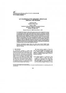
This method relies on coding the data stored in the memory, is slightly slower than the conventional approach when learning, but is just as quick in analyse mode. The method proposed uses m-bit wide memory to discriminate between 2" - 2 classes, whereas m-discriminators (which can be considered to be one discriminator m-bits wide) can discriminate only m-classes. This can be a significant saving; for example, 3-bit wide memory will recognise 6 objects, so the a m o u n t of memory required is halved, 4-bit wide memory will recognise 14 objects and 5-bit wide memory will recognise 30 objects. In the proposed method, the same memory is used for all the different objects, but the value stored in each location is unique to each object. Thus, the binary number r is stored when object r is learnt. However, the analysis of two different objects may generate the same address. Therefore, a separate number is written there to indicate such a clash. Another number, G R O U N D , is needed to indicate uninitialised data. This is similar to the method used in the auto-associative network described above. On analysing a new object, the addresses are formed in the standard way, and a count is made of the numbers found at the addresses. The number found most often is identified as the object, and the two measures of confidence given earlier can still be used. The algorithms are: Initially: Load each location with the G R O U N D value. On learnin9 object r: For any generated address (that is the tuple value and its number) IF data at address -- G R O U N D T H E N Store r at that address E L S E I F data ( ) r T H E N store CLASH at that address On analysin9 an object: Set the number of 'fires' for each object to 0. For each generated address, Read the value at that address; 1F value ( ) G R O U N D A N D value ( ) CLASH T H E N Increment 'fire' count for that value.

560

R.J. Mitchell et aLlMathematics and Computers in Simulation 40 (1996) 549-563

Input

Randomiser

m-bit RAMS

Randomiser v

m-bit RAMS

Demulti-

.

.

.

.

.

.

plexor

Demultiplexor

Fig. 9. Block diagram of ‘coded memory’ system.

Note, the method can only be used with discriminators using the same tuple sampling sequence. A block diagram implementing the system is shown in Fig. 9. This contains various discriminators, each m-bit wide. In analyse mode, the value output from the discriminator, that is the number of the class found in the neuron, is used to select the particular counter to be incremented; a standard demultiplexor circuit achieves this selection. Thus the method can easily be implemented in hardware. 7.3. The saturation problem The standard n-tuple method requires that similar versions of the object are learnt many times, so that when a new version of the object is shown to the system, although it is not identical to one already seen, it is sufficiently similar. Care is required, however, to ensure that the memory is not filled too much, as then the system will ‘recognise’ objects it was not taught. This is the saturation problem. In the proposed method a greater proportion of the memory is used, so there is a greater danger of saturation. A measure of saturation can be found by noting the number of clashes. A clash occurs when two different objects are sufficiently similar that the same address is generated when they are analysed, and these are more likely to occur when more versions of an object are learnt. Hence fewer versions of each object should be taught to the system than for a standard network, and so the proposed system will be less able to distinguish between similar objects than the standard method. However, experimental results have shown that the performance is not affected too much. One reason why extra learning is required is to handle noise distorted data. If the input were filtered using, say, an auto-associative network, before being passed to the recognition network, then the amount of learning required would be reduced.

8. Experiments The test data used to evaluate the performance of the system are the images of various characters. A number of such sets of characters have been used, of size 8 x 8,16 x 16 and 32’x 32 dots. A simple

R.J. Mitchell et al./Mathematics and Computers in Simulation 40 (1996) 549-563

561

program has been written, using the network development environment O R T H A N C [21] which compares the performance of the proposed system with that of the standard method. The program allows the user to select the character set under consideration, which of the characters are to be analysed, the tuple size and whether random or sequential addressing of the input pattern (mapping) is needed. Practical tests show that a tuple size of 8 and random mapping are optimal, as is well documented [1], and these are used throughout. When data are learnt, the user specifies the seed of the random number generator used to form tuples (to allow different mapping of the objects) and the amount of learning done. The system learns the 'pure' object and a user selected number of the versions of the object at Hamming distance of 1 from the 'pure' version. The performance of the system is then evaluated by showing the system distorted versions of the objects and calculating the confidence levels and the number of erroneous classifications.

9. Results and discussion Fig. 10 shows some typical results for both the standard and the proposed systems. For these, the data sets were the ten decimal digits of image size 32 x 32, and the graphs show the response when distorted amounts of characters 4, 0 and 8 were input: these were chosen as they give the best, average and worst performance of the ten digits. The absolute confidence of the proposed system is worse than that of the standard method, but the relative confidence is better. However, the number of classification errors (where the system classified the character incorrectly, or could not determine the character as no single character had the most 'fires') is increased slightly; for the examples shown, only 8 is misclassified. The reason for the higher-relative confidence measure is as follows. When a character is shown to a standard network, it is likely that many discriminators will fire. Typical values for the 'most number of fires' and the 'next most' for 32 x 32 images and tuple size of 8, are 18 and 5 respectively, giving a relative confidence of 72%. However, for the proposed networks there are fewer 'fires' for each character, because of clashes, so typical values for 'most number of fires' and 'next most' are 9 and 1, for which the relative confidence is 89%. The fewer number of 'fires' for the proposed system can produce problems. If the different objects being taught are too similar, clashes can occur so often that for some data the number of 'fires' is zero. For example, for one set of decimal digits of size 8 x 8 used, character 8 was too similar to the other characters, so that even when pure images only were taught, the tuples formed for 8 always resulted in 'clash' being stored in the discriminator. The system was, however, able to learn and distinguish between the characters 1 2 4 5 6 and 7. In general it was found that the system was better at classifying objects when larger images were used, although the absolute and relative confidences were not affected much by size. Again this is because of clashes. For a smaller image there are fewer tuples, so fewer 'fires' are possible and so clashes are more likely to reduce the count of 'fires' to zero, than for larger images. One method by which the number of tuples formed could be increased is to over sample. That is, instead of sampling the image so that each element is used only once, the system could sample the pattern so each element is sampled many times. The disadvantage of this is that it requires more memory. However, tests showed that this resulted in fewer classification errors.

562

R.J. Mitchell et aLlMathematics and Computers in Simulation 40 (1996) 549-563

ProposedSystem

StandardSystem 100 %AbsoluteConfidence 1

I

1oo %AbsoluteConfidence I

_

_

3

6

.

9

.

‘

12

15

3

6

3

6

9 12 15 % distortion

9

12

15

% distortion

% distortion

3

6

9

12

15

0 distortion

Fig. 10. Typical results of coded memory system.

10. Conclusion This paper has considered the memory requirements of the n-tuple or weightless form of neural network. In so doing, the principles behind these networks have been demonstrated, some configurations of networks discussed, and its hardware implementation considered. One problem with these networks is that large amounts of memory may be required, particularly when processing many data classes. An auto-associative system is discussed which requires less memory. Then a novel system is proposed for multiple object n-tuple recognition systems. The

R.J. Mitchell et al./M athematics and Computers in Simulation 40 (1996) 549-563

563

response of this system is shown to be similar to the standard method, but requiring less memory. However, the system response is shown to be affected when different data classes are too similar and by the size of the data patterns.

References [1] I. Aleksander and T.J. Stonham, A guide to pattern recognition using random access memories, IEE Proc. E, Comput. Digital Tech. 2(1) (1979) 29-40. 1,2] I. Aleksander and H. Morton, An Introduction to Neural Computing (Chapman & Hall, London, 1990). [3] D.E. Rumelhart and J.L. McClelland, Parallel Distributed Computing, Vol. 1 (MIT Press, Cambridge, MA, 1986). [4] T. Kohonen, Self Organisation and Associative Memory (Springer, Berlin, 1984). [5] J.J. Hopfield, Neural networks and physical system with emergent collective properties, Proc. Nat. Acad. Sci. USA 79 (1982) 2554-2558. [6] G.E. Hinton, T.J. Sejnowski and D.H. Ackley, Boltzmann machines: Constraint satisfaction networks that learn, Technical Report No. CMU-CS-84-119, 1984. I-7] I. Aleksander, ed., Neural Computing Architectures (North Oxford Academic Publishers, 1989). [8] D. Aitken, J.M. Bishop, R.J. Mitchell and S.E. Pepper, Pattern separation using digital learning nests, Electron Lett. 25(11) (1989) 685-686. I-9] I. Aleksander and R.C. Albrow, Micro-circuit learning nets: Some tests with handwritten numerals, Electron. Lett. 4(19) (1968) 406-407. 1,10] T.J. Stonham and I. Aleksander, Automatic classification of mass spectra by means of digital learning nets, Electron. Lett. 9(17) (1973) 391-394. [11] J.M. Bishop, Anarchic techniques for pattern classification, Ph.D. Thesis, Reading University, 1989. [12] D.E. Goldberg, Genetic Algorithms (Addison-Wesley, Reading, MA, 1989). [13] J.M. Bishop, A.A. Crowe, P.R. Minchinton and R.J. Mitchell, lEE Colloq. on Machine Learning, Digest 1990/117, 1990. [14] J.M. Bishop, P.R. Minchinton and R.J. Mitchell, Multi class pattern association using digital n-tuple networks, Proc. INNC-90-Paris (1990) p. 926. [15] J.M. Bishop, P.R. Minchinton and R.J. Mitchell, Auto-associative digital neural network for grey level data, Proc. ICANN 92 (1992) pp. 639-642-8. [16] I. Aleksander, W.V. Thomas and P.A. Bowden, WlSARD, a radical step forward in image recognition, Sensor Rev. 4 (1984). 1-17] R.J. Mitchell, P.R. Minchinton, J.P. Brooker and J.M. Bishop, A modular weightless neural network system, Proc. ICANN 92, Artificial Neural Networks 2 (1992) 635-638. [18] R.J. Mitchell, P.R. Minchinton, J.M. Bishop, J.W. Day, J.F. Hawker and S.K. Box, Modular hardware weightless neural networks, Proc. Weightless Neural Networks Workshop '93 (1993) pp. 123-128. [19] R. Rohwer and A.Y. Lamb, An exploration of the effect of super large n-tuples on single layer ramnets, Proc. Weightless Neural Networks Workshop '93 (1993) pp. 33-37. [20] R. Patel and R. O'Hagan, DNA finger print matching, Neural Network Project Report, Department of Cybernetics, 1993. [21] J.M. Bishop, P.R. Minchinton and R.J. Mitchell, O R T H A N C - An n-tuple network development environment, Proc. INNC-90-Paris (1990) pp. 685-688.