formance Testing (HPT) framework for performance com- parison ... statistical methods (such as the paired -test or confidence interval) ... cal performance testing framework. Section 5 ...... Later, in the context of Java performance evalua-.
Statistical Performance Comparisons of Computers∗ Tianshi Chen†§ , Yunji Chen†§ , Qi Guo† , Olivier Temam‡ , Yue Wu† , Weiwu Hu†§ † State Key Laboratory of Computer Architecture, Institute of Computing Technology, Chinese Academy of Sciences, Beijing, China ‡ INRIA, Saclay, France § Loongson Technologies Corporation Limited, Beijing, China Abstract As a fundamental task in computer architecture research, performance comparison has been continuously hampered by the variability of computer performance. In traditional performance comparisons, the impact of performance variability is usually ignored (i.e., the means of performance measurements are compared regardless of the variability), or in the few cases where it is factored in using parametric confidence techniques, the confidence is either erroneously computed based on the distribution of performance measurements (with the implicit assumption that it obeys the normal law), instead of the distribution of sample mean of performance measurements, or too few measurements are considered for the distribution of sample mean to be normal. We first illustrate how such erroneous practices can lead to incorrect comparisons. Then, we propose a non-parametric Hierarchical Performance Testing (HPT) framework for performance comparison, which is significantly more practical than standard parametric techniques because it does not require to collect a large number of measurements in order to achieve a normal distribution of the sample mean. This HPT framework has been implemented as an open-source software.
1
Introduction
A fundamental practice for researchers, engineers and information services is to compare the performance of two ∗ T. Chen, Y. Chen, Q. Guo, and W. Hu are partially supported by the National Natural Science Foundation of China (under Grants 61100163, 61003064, 61173006, 61133004, 60736012, and 60921002), the National S&T Major Project of China (under Grants 2009ZX01028-002-003, 2009ZX01029-001-003, and 2010ZX01036-001-002), and the Strategic Priority Research Program of the Chinese Academy of Sciences (under Grant XDA06010400). O. Temam is supported by HiPEAC-2 NoE under Grant European FP7/ICT 217068 and INRIA YOUHUA.
978-1-4673-0825-0/12/$31.00 ©2012 IEEE
architectures/computers using a set of benchmarks. As trivial as this task may seem, it is well known to be fraught with obstacles, especially the selection of benchmarks [31, 33, 3] and performance variability [1]. In this paper, we focus on the issue of performance variability. The variability can have several origins, such as non-deterministic architecture+software behavior [6, 26], performance measurement bias [27], or even applications themselves. Whatever the origin, the performance variability is well known to severely hamper the comparison of computers. For instance, the geometric mean performance speedups, over an initial baseline run, of 10 subsequent runs of SPLASH-2 on a commodity computer (Linux OS, 4-core 8-thread Intel i7 920 with 6 GB DDR2 RAM) are 0.94, 0.98, 1.03, 0.99, 1.02, 1.03, 0.99, 1.10, 0.98, 1.01. Even when two computers/architectures may have fairly different performance, such variability can still make the quantitative comparison (e.g., estimating the performance speedup of one computer over another) confusing or plain impossible. Incorrect comparisons can, in turn, affect research or acquisition decisions, so the consequences are significant. The most common and intuitive way of addressing the impact of variability is to compute the confidence of performance comparisons. The most broadly used techniques for estimating the confidence are parametric confidence estimate techniques [1, 27]. However, at least two kinds of wrongful practices commonly plague the usage of such techniques, potentially biasing performance comparisons, and consequently, sometimes leading to incorrect decisions. The first issue is that computing a confidence based on a statistical distribution implicitly requires that distribution to be normal. However, the Central Limit Theorem (CLT) [4] says that, even if a distribution of performance measurements is not normal, the distribution of the sample mean (a sample is simply a set of performance measurements) tends to a normal distribution as the sample size (the number of measurements in each sample) increases. The problem, though, is that the confidence estimate is often erro-
neously based on the distribution of performance measurements (with the implicit assumption that it obeys the normal law), instead of the distribution of the sample mean. That wrongful practice could still lead to a correct estimate of the confidence if the distribution of performance measurements is, by chance, normal, but we will empirically show that the distribution of performance measurements can easily happen to be non-normal, so that such erroneous usage of the confidence estimate is harmful. The second issue is that, even if parametric confidence estimate techniques are correctly based on the distribution of the sample mean, the number of measurements collected is usually insufficient to achieve a normally distributed sample mean. In day-to-day practices in computer architecture research, such techniques are commonly applied when about 30 performance measurements have been collected. However, we will empirically show that a very large number of performance measurements, on the order of 160 to 240, are required for the CLT to be applicable, so that current practices can again lead to harmful usage of the parametric techniques. In this paper, we introduce the Hierarchical Performance Test (HPT) which can correctly quantify the confidence of a performance comparison even if only a few performance measurements are available. The key insight is to use nonparametric Statistic Hypothesis Tests (SHTs). Parametric statistical methods (such as the paired 𝑡-test or confidence interval) rely on some distribution assumptions, while the non-parametric SHTs quantify the confidence using data rankings. Non-parametric SHTs can work when there are only a few performance measurements, because they do not need to characterize any specific distribution. To help disseminate the use of non-parametric SHTs, we design a selfcontained Hierarchical Performance Test (HPT) and the associated software implementation, which will be openly distributed. In summary, the contributions of this paper are the following. First, we empirically highlight that traditional performance comparisons simply based on means of performance measurements can be unreliable because of the variability of performance results. As a result, we stress that every performance comparison should come with a confidence estimate in order to judge whether a comparison result corresponds to a stochastic effect or whether it is significant enough. Second, we provide quantitative evidence that two common wrongful practices, i.e., using the distribution of performance measurements instead of the distribution of sample mean, and using too few performance measurements, are either harmful or render parametric confidence techniques impractical for our domain. Third, we propose and implement the HPT framework based on nonparametric SHTs, which can provide a sound quantitative estimate of the confidence of a comparison, independently
of the distribution and the number of performance measurements. The rest of the paper is organized as follows. Section 2 motivates the need for systematically assessing the confidence of performance measurements, and for using the appropriate statistical tools to do so. Section 3 investigates the impact of using the wrong distribution or of collecting an insufficient number of performance measurements for the normality assumption of parametric confidence techniques. Section 4 introduces the non-parametric hierarchical performance testing framework. Section 5 empirically compares the HPT with traditional performance comparison techniques. Section 6 reviews the related work.
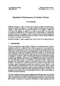
2 Motivation In this section, we introduce two examples to motivate this study. The first example shows the significance of using statistical techniques in performance comparisons, and the second example shows the importance of selecting appropriate statistical techniques. In a quantitative performance comparison, the performance speedup of one computer over another is traditionally obtained by comparing the geometric mean performance of one computer (over different benchmarks) with that of another, a practice adopted by SPEC.org [31]. Following this methodology, the performance speedup of PowerEdge T710 over Xserve on SPEC CPU2006, estimated by the data collected from SPEC.org [31], is 3.50. However, after checking this performance speedup with the HPT proposed in this paper, we found that the confidence of such a performance speedup is only 0.31, which is rather unreliable (≥ 0.95 is the statistically acceptable level of confidence). In fact, our HPT reports that the reliable performance speedup is 2.24 (with a confidence of 0.95), implying that the conclusion made by comparing geometric mean performance of two computers brings an error of 56.2% for the quantitative comparison. Let us now use another example to briefly illustrate why using parametric confidence techniques incorrectly can be harmful. In this section we emulate the wrongful practice of computing the confidence based on the distribution of performance measurements, instead of the distribution of sample mean. We consider the quantitative performance comparison of another pair of commodity computers, Asus P5E3 Premium and CELSIUS R550. In Figure 1, we show the histograms of the SPEC ratios of the two computers (collected from SPEC.org). Clearly, neither of the histograms appears to correspond to a normal distribution. We further evaluated the normality of the distributions using the Lilliefors test (Kolmogorov-Smirnov test) [24], and we found that, for both computers, the normality assumption is indeed incorrect for confidences larger than 0.95.
6
8
5 4
Asus P5E3 Premium (Intel Core 2 Extreme QX9770)
3 2
Frequency
Frequency
6
CELSIUS R550 (Intel Xeon E5440 processor)
4
2 1 0
50
100
SPEC Ratio
150
0
50
100
150
200
SPEC Ratio
Figure 1. Histograms of SPEC ratios of two commodity computers.
Voluntarily ignoring that observation, we incorrectly use the confidence interval based on the non-normal distribution of performance measurements for the quantitative comparison. The confidence interval technique says that Asus P5E3 Premium is more than 1.02 times faster than CELSIUS R550 with a confidence of 0.95, and 1.15 times faster with a confidence of 0.12. According to the HPT, the Asus P5E3 Premium is actually more than 1.15 times faster than the CELSIUS R550 with a confidence of 0.95. So the confidence of the claim “Asus P5E3 Premium is 1.15 times faster than CELSIUS R550” is drastically under-evaluated (0.12 instead of 0.95), or conversely, the assessment of the speedup for a fixed confidence of 0.95 is again largely under-evaluated (1.02 instead of 1.15). In summary, it is important not only to assess the confidence of a performance comparison, but also to correctly evaluate this confidence.
3
Issues with Current Performance Comparison Practices
In this section, we empirically highlight that the distribution of performance measurements may not be normal, and thus it cannot be used to directly compute the confidence. Then, we empirically again show that a large number of measurements are required in order to use the Central Limit Theorem (CLT).
3.1
Checking the Normality of Performance Measurements
To compare the performance of different computers, we expect that the performance score on each benchmark can stably reflect the exact performance of each computer. However, the performance of a computer on every benchmark is influenced by not only architecture factors (e.g., out-of-order execution, branch prediction, and chip multiprocessor [34]) but also program factors (e.g., data race, synchronization, and contention of shared resources [2]). In the presence of these factors, the performance score of a
computer on a benchmark is usually a random variable [1]. For example, according to our experiments using SPLASH2 [33], the execution time of one run of a benchmark can be up to 1.27 times that of another run of the same benchmark on the same computer. Therefore, it is necessary to provide some estimate of the confidence of a set of computer performance measurements. As mentioned before, the confidence is sometimes incorrectly assessed based on the distribution of performance measurements, which can only lead to a correct result if that distribution is normal. We empirically show that this property is not valid for the following set of rather typical performance measurements. In our experiments, we run both single-threaded (Equake, SPEC CPU2000 [31]) and multi-threaded benchmarks (Raytrace, SPLASH-2 [33] and Swaptions, PARSEC [3]) on a commodity Linux workstation with a 4-core 8-thread CPU (Intel i7 920) and 6 GB DDR2 RAM. Each benchmark is repeatedly run for 10000 times, respectively. At each run, Equake uses the “test” input defined by SPEC CPU2000, Raytrace uses the largest input given by SPLASH-2 (car.env), and Swaptions uses the second largest input of PARSEC (simlarge). Without losing any generality, we define the performance score to be the execution time. To check the normality of the performance, we empirically study whether the normal Probability Density Function (PDF) obtained by assuming the normality of the execution time complies with the real PDF of the execution time. In our experiments, we utilize two statistical techniques, Naive Normality Fitting (NNF) and Kernel Parzen Window (KPW) [28]. The NNF technique assumes that the execution time obeys a normal law and estimates the corresponding normal distribution, while the KPW technique provides the real distribution of the execution time without assuming a normal distribution. If the normal distribution obtained by the NNF complies with the real distribution estimated by the KPW, then the performance score obeys a normal law. Otherwise, it does not. Statistically, the NNF technique directly employs the mean and deviation of the sample (with 10000 measurements of the execution time) as the mean and standard deviation of the normal distribution. In contrast, without assuming the normality, the KPW technique estimates the real distribution of the execution time in a Monte-Carlo style. It estimates directly the probability density at each point via histogram construction and Gaussian kernel smoothing. By comparing the PDFs obtained by the two techniques, we can easily identify whether or not the distribution of performance measurements obeys a normal law. According to the experimental results illustrated in Figure 2, the normality does not hold for the performance score of the computer on all three benchmarks, as evidenced by the remarkably long right tails and short left tails of the
−3
x 10
−4
Equake, SPEC CPU2000 (10000 Runs)
1.4
x 10
−4
Raytrace, SPLASH−2 (10000 Runs)
1.6
x 10
Swaptions, PARSEC (10000 Runs)
1.2 1.4
1.2
Sample Mean
0.6 0.4 0.2 0 2.18
1
Probability Density
Probability Density
Probability Density
0.8
Sample Mean
Sample Mean
1
0.8 0.6 0.4 0.2
2.2
2.22
2.24
2.26
Execution Time (us)
2.28
2.3 5
x 10
0 5.41
1.2 1 0.8 0.6 0.4 0.2
5.61
5.81
6.01
6.21
6.41
6.61
Execution Time (us)
6.8
0 6.3
6.8
7.3
7.8
8.3
Execution Time (us)
5
x 10
8.6 5
x 10
Figure 2. Estimating Probability Density Functions (PDFs) on Equake (SPEC CPU2000), Raytrace (SPLASH-2) and Swaptions (PARSEC) by KPW (black curves above the grey areas) and NNF (black curves above the white areas), from 10000 repeated runs of each benchmark on the same computer.
score obeys the normality law. Figure 3 illustrates the normal probability plot [5] for the performance of a commodity computer (4-Core Intel Core i7-870, Intel DP55KG motherboard), where the data is collected from the SPEC online repository [31]. In each probability plot presented in Figure 3, if the curve matches well the straight line, then the performance distributes normally over the corresponding benchmark suite; if the curve departs from the straight line, then the performance does not distribute normally. Obviously, neither of the figures shows a good match between the curve and straight line, implying that the performance of the computer does not distribute normally over both SPECint2006 and SPECfp2006.
Probability
0.95 0.90
Probability
estimated performance distributions for Equake, Raytrace and Swaptions. Such observations are surprising but not counter-intuitive due to the intrinsic non-determinism of computers and applications. Briefly, it is hard for a program to execute faster than a threshold, but easy to be slowed down by various events, especially for multi-threaded programs which are affected by data races, thread scheduling, synchronization order, and contentions of shared resources. As a follow-up experiment, we use a more rigorous statistical technique to study whether the execution times of the 27 benchmarks of SPLASH-2 and PARSEC (using “simlarge” inputs) distribute normally; each benchmark is repeatedly run on the commodity computer for 10000 times again. Based on these measurements, the Lilliefors test (Kolmogorov-Smirnov test) [24] is utilized to estimate the confidence that the execution time does not obey the normal law, i.e., the confidence that the normality assumption is incorrect. Interestingly, it is observed that for every benchmark of SPLASH-2 and PARSEC, the confidence that the normality assumption is incorrect is above 0.95. Our observation with SPLASH-2 and PARSEC is significantly different from the observation of Georges et al. [12] that single-benchmark performance on single cores (using SPECjvm98) distributes normally, suggesting that the performance variability of multi-threaded programs is fairly different from that of single-threaded programs. In fact, the same can be observed for the performance variability of a computer over a set of different benchmarks. Considering the performance score of a computer which may vary from one benchmark to another, we empirically study whether the distribution of the performance
0.75 0.50 0.25 0.10 0.05
SPECint2006 50
100
150
SPEC Ratio
200
0.98 0.95 0.90 0.75 0.50 0.25 0.10 0.05 0.02
SPECfp2006 30
40
50
60
70
SPEC Ratio
Figure 3. Graphically assessing whether the performance measurements of a commodity computer distribute normally (normal probability plots [5]) using performance scores (SPEC ratios) for SPECint2006 and SPECfp2006. Finally, we use the Lilliefors test [24] to analyze the data of 20 other commodity computers randomly selected from the SPEC online repository [31]. Using the whole
SPEC CPU2006 suite, all 20 computers exhibit non-normal performance with a confidence larger than 0.95. For SPECint2006, 19 out of 20 computers exhibit non-normal performance with a confidence larger than 0.95, and for SPECfp2006, 18 out of 20 computers exhibit non-normal performance with a confidence larger than 0.95. So we can consider that, in general, the distribution of performance measurements does not obey the normal law, and thus, it should never be used to directly estimate the confidence of these measurements with parametric techniques. Only the distribution of the sample mean should be used, as stated by the Central Limit Theorem.
3.2
Checking the Applicability of the Central Limit Theorem
So far we have empirically shown that the performance of computers cannot be universally characterized by normal distributions. However, it is still possible to obtain a normally distributed mean of performance measurements (in order to apply parametric techniques) given a sufficiently large number of measurements, as guaranteed by the Central Limit Theorem. More specifically, let {𝑥1 , 𝑥2 , . . . , 𝑥𝑛 } be a size-𝑛 sample consisting of 𝑛 measurements of the same non-normal distribution with mean 𝜇 and finite vari∑𝑛 ance 𝜎 2 , and 𝑆𝑛 = ( 𝑖=1 𝑥𝑖 )/𝑛 be the mean of the measurements (i.e., sample mean). According to the classical version of the CLT contributed by Lindeberg and L´evy [4], when the sample size 𝑛 is sufficiently-large, the sample mean approximately obeys a normal distribution. Nevertheless, in practice, it is unclear how large the sample size should be to address the requirement of “a sufficiently large sample”. In this section, we empirically show that the appropriate sample size for applying the CLT is usually too large to be compatible with current practices in computer performance measurements. In order to obtain a large number performance measurements, we use the KDataSets [7]. A notable feature of KDataSets is that it provides 1000 distinct data sets for each of 32 different benchmarks (MiBench [14]), for a total of 32,000 distinct runs. We collect the detailed performance scores (performance ratios normalized to an ideal processor executing one instruction per cycle) of a Linux workstation (with 3GHz Intel Xeon dualcore processor, 2GB RAM) over the 32,000 different combinations of benchmarks and data sets of KDataSets [7]. In each trial, we fix the number of different samples to 150, leading to 150 observations of sample mean, which are enough to obtain a normal distribution as predicted by the CLT [15]. In order to construct each sample, we randomly select 𝑛 performance scores out of the 32,000 performance scores, where the sample size 𝑛 (i.e., number of measurements) is varied from 10 to 280 by increments of 20. For each trial with a fixed sample
size, we estimate the probability distribution of the sample mean via the statistical technique called Kernel Parzen Window (KPW) [28]. Technically, the KPW has a parameter called “window size” or “smoothing bandwidth”, which determines how KPW will smooth the distribution curve. In general, the larger the window size, the smoother the curve. But if we choose a too large window size, there is a risk that a non-normal curve is rendered as normal by KPW. In order to avoid that, in each trial we start from a small window size, and we increase it until the distribution curve becomes smooth enough. After that, we judge whether the distribution has approached a normal distribution by checking if it is symmetric with respect to its center. The different probability distributions over the 15 trials are illustrated in Figure 4. Clearly, the sample mean does not distribute normally given a small (e.g., 𝑛 = 10 − 140) sample size. When the sample size becomes larger than 240, the distribution of the mean performance seems to be a promising approximation of a normal distribution. In addition, we further carry out the Lilliefors test for each trial, and we find that the mean performance does not distribute normally when 𝑛 < 160. The above observation implies that at least 160 to 240 performance measurements are necessary to make the CLT and parametric techniques applicable, at least for this benchmark suite. However, such a large number of performance measurements can rarely be collected in day-to-day practices; most computer architecture research studies rely on a few tens of benchmarks, with one to a few data sets each, i.e., far less than the aforementioned number of required performance measurements. In order to cope with a small number of performance measurements, we propose to use a non-parametric statistical framework.
4
Non-parametric Hierarchical Performance Testing Framework
Statistical inference techniques are popular for decision making processes based on experimental data. One crucial branch of statistical inference is called Statistical Hypothesis Test (i.e., SHT). More specifically, an SHT is a procedure that makes choices between two opposite hypotheses (propositions), the NULL (default) hypothesis and the alternative hypothesis. The NULL hypothesis represents the default belief, i.e., our belief before observing any evidence, and the alternative hypothesis (often the claim we want to make) is a belief opposite to the NULL hypothesis. In performance comparison, a typical NULL hypothesis may be “computer 𝐴 is as fast as computer 𝐵”, and a typical alternative hypothesis may be “computer 𝐴 is faster than computer 𝐵”. At the beginning of an SHT, one assumes the NULL hypothesis to be correct, and constructs a statistic (say, 𝑍) whose value
10
n=10
5
10
n=20
5 0 20
1.4 1.6 1.8
2
2.2
n=100
5
0 1.4 20
1.6
1.8
2
n=120
10
1.7
1.8
1.9
n=200
1.7
1.8
1.9
n=220
10
1.7
1.8
1.9
2
2.2
0 1.6
1.7
1.8
1.9
1.8
1.9
1.8
2
0 1.6
1.8
1.9
1.7
1.8
1.9
1.8
1.9
1.8
1.9
10
0 1.6 20
1.7
1.8
1.9
0 1.6
0 1.6 20
1.7
n=280
10
1.7
0 1.6 20
n=180
n=260
10
1.7
0 1.6 20 10
0 1.6 20
n=80
10
n=160
n=240
10
0 1.6
0 1.4 1.6 1.8 20 10
0 1.6 20
20
n=60
5
n=140
10
0 1.6 20
10
n=40
10
1.7
1.8
1.9
0 1.6
1.7
Figure 4. How many performance measurements are required to construct a sufficiently-large sample? can be calculated from the observed data. The value of 𝑍 determines the possibility that the NULL hypothesis holds, which is critical for making a choice between the NULL hypothesis and the alternative hypothesis. The possibility that the NULL hypothesis does hold is quantified as the socalled 𝑝-𝑣𝑎𝑙𝑢𝑒 (or significance probability) [21], which is a real value between 0 and 1 that can simply be considered as a measure of risk associated with the alternative hypothesis. The 𝑝-𝑣𝑎𝑙𝑢𝑒 is an indicator for decision-making: when the 𝑝-𝑣𝑎𝑙𝑢𝑒 is small enough, then the risk of incorrectly rejecting the NULL hypothesis is very small, and the confidence of the alternative hypothesis (i.e., 1 − 𝑝-𝑣𝑎𝑙𝑢𝑒) is large enough. For example, in an SHT, when the 𝑝-𝑣𝑎𝑙𝑢𝑒 of the NULL hypothesis “computer 𝐴 is as fast as computer 𝐵” is 0.048, we only have a 4.8% chance of rejecting the NULL hypothesis when it actually holds. In other words, the alternative hypothesis “computer 𝐴 is faster than computer 𝐵” has confidence 1−0.048 = 0.952. Closely related to the 𝑝-𝑣𝑎𝑙𝑢𝑒, the significance level acts as a scale of the ruler for the 𝑝-𝑣𝑎𝑙𝑢𝑒 (frequently-used scales include 0.001, 0.01, 0.05, and 0.1). A significance level 𝛼 ∈ [0, 1], can simply be viewed as the confidence level 1 − 𝛼. As a statistical convention, a confidence no smaller than 0.95 is often necessary for reaching the final conclusion. Among the most famous and broadly used SHTs, many are parametric ones which rely on normally distributed means of measurements. In the rest of this section, we introduce a Hierarchical Performance Testing (HPT) framework, which integrates non-parametric SHTs for performance comparisons.
4.1
General Flow
Concretely, the HPT employs Wilcoxon Rank-Sum Test [35] to check whether the difference between the performance scores of two computers on each benchmark is significant enough (i.e., the corresponding significance level is
small enough), in other words, whether the observed superiority of one computer over another is reliable enough. Only significant (reliable) differences, identified by the SHTs in single-benchmark comparisons, can be taken into account by the comparison over different benchmarks, while those insignificant differences will be ignored (i.e., the insignificant differences are set to 0) in the comparison over different benchmarks. Based on single-benchmark performance measurements, the Wilcoxon Signed-Rank Test [9, 35] is employed to statistically compare the general performance of two computers. Through these non-parametric SHTs, the HPT can quantify the confidence for performance comparisons. In this section, the technical details of the HPT will be introduced. 1 Let us assume that we are comparing two computers 𝐴 and 𝐵 over a benchmark suite consisting of 𝑛 benchmarks. Each computer repeatedly runs each benchmark 𝑚 times (𝑚 ≥ 3). Let the performance scores of 𝐴 and 𝐵 at their 𝑗-th runs on the 𝑖-th benchmark be 𝑎𝑖,𝑗 and 𝑏𝑖,𝑗 respectively. Then the performance samples of the computers can be represented by performance matrices 𝑆𝐴 = [𝑎𝑖,𝑗 ]𝑛×𝑚 and 𝑆𝐵 = [𝑏𝑖,𝑗 ]𝑛×𝑚 , respectively. For the corresponding rows of 𝑆𝐴 and 𝑆𝐵 (e.g., the 𝜏 -th rows of the matrices, 𝜏 = 1, . . . , 𝑛), we carry out the Wilcoxon Rank-Sum Test to investigate whether the difference between the performance scores of 𝐴 and 𝐵 is significant enough. The concrete steps of Wilcoxon Rank-Sum Test are the following: ∙ Let the NULL hypothesis of the SHT be “𝐻𝜏,0 : the performance scores of 𝐴 and 𝐵 on the 𝜏 -th benchmark are equivalent to each other”; let the alternative hypothesis of the SHT be “𝐻𝜏,1 : the performance score of 𝐴 is higher than that of 𝐵 on the 𝜏 -th benchmark” or “𝐻𝜏,2 : the performance score of 𝐵 is higher than that of 𝐴 on the 𝜏 -th benchmark”, depending on the motivation of carrying out 1 Users who are not interested in the mathematical details of the nonparametric SHTs can omit the rest of this subsection.
the SHT. Define the significance level be 𝛼𝜏 ; we suggest setting 𝛼𝜏 = 0.05 for 𝑚 ≥ 5 and 0.10 for the rest cases. ∙ Sort 𝑎𝜏,1 , 𝑎𝜏,2 , . . . , 𝑎𝜏,𝑚 , 𝑏𝜏,1 , 𝑏𝜏,2 , . . . , 𝑏𝜏,𝑚 in ascending order, and assign each of the scores the corresponding rank (from 1 to 2𝑚). In case two or more scores are the same, but their original ranks are different, then renew the ranks by assigning them the average of their original ranks2 . Afterwards, for A and B, we can define their rank sums (on the 𝜏 -th benchmark) to be: R𝑎,𝜏 =
𝑚 ∑
Rank𝜏 (𝑎𝜏,𝑗 ),
𝑗=1
R𝑏,𝜏 =
𝑚 ∑
Rank𝜏 (𝑏𝜏,𝑗 ),
𝑗=1
where Rank𝜏 (⋅) provides the rank of a performance score on the 𝜏 -th benchmark. ∙ Case[𝑚 < 12]3 : When the alternative hypothesis of the SHT is 𝐻𝜏,1 , we reject the NULL hypothesis and accept 𝐻𝜏,1 if R𝑎,𝜏 is no smaller than the critical value (right tail, Wilcoxon Rank-Sum Test) under the significance level 𝛼𝜏 . When the alternative hypothesis of the SHT is 𝐻𝜏,2 , we reject the NULL hypothesis and accept 𝐻𝜏,2 if R𝑏,𝜏 is no smaller than the critical value under the significance level 𝛼 [15]. ∙ Case[𝑚 ≥ 12]: Define two new statistics 𝑧𝑎,𝜏 and 𝑧𝑏,𝜏 as follows: 𝑧𝑎,𝜏 =
R𝑎,𝜏 − 12 𝑚(2𝑚 + 1) √ , 1 𝑚2 (2𝑚 + 1) 12
𝑧𝑏,𝜏 =
R𝑏,𝜏 − 12 𝑚(2𝑚 + 1) √ . 1 𝑚2 (2𝑚 + 1) 12
Under the NULL hypothesis, 𝑧𝑎,𝜏 and 𝑧𝑏,𝜏 approximately obey the standard normal distribution 𝒩 (0, 1). When the alternative hypothesis of the SHT is 𝐻𝜏,1 , we reject the NULL hypothesis and accept 𝐻𝜏,1 if 𝑧𝑎,𝜏 is no smaller than the critical value (right tail, standard normal distribution) under the significance level 𝛼; when the alternative hypothesis of the SHT is 𝐻𝜏,2 , we reject the NULL hypothesis and accept 𝐻𝜏,2 if 𝑧𝑏,𝜏 is no smaller than the critical value under the significance level 𝛼 [15]. After carrying out the above SHT with respect to the 𝜏 -th benchmark (𝜏 = 1, . . . , 𝑛), we are able to assign the difference (denoted by 𝑑𝜏 ) between the performance of 𝐴 and 𝐵. Concretely, if the SHT accepts 𝐻𝜏,1 or 𝐻𝜏,2 with a promising significance level (e.g., 0.01 or 0.05), then we let 𝑑𝜏 = median{𝑎𝜏,1 , 𝑎𝜏,2 , . . . , 𝑎𝜏,𝑚 } −median{𝑏𝜏,1 , 𝑏𝜏,2 , . . . , 𝑏𝜏,𝑚 },
𝜏 = 1, . . . , 𝑛.
Otherwise (if the NULL hypothesis 𝐻𝜏,0 has not been rejected at a promising significant level), we let 𝑑𝜏 = 0, i.e., 2 For example, if two scores are both 50, and their original ranks are 5 and 6 respectively, then both of them obtain a rank of 5.5. 3 In statistics, when 𝑚 < 12, the critical values for Wilcoxon rank sum test are calculated directly. When 𝑚 ≥ 12, the corresponding critical values are often estimated by studying the approximate distribution of the rank sum.
we ignore the insignificant difference between the performance scores of 𝐴 and 𝐵. 𝑑1 , 𝑑2 , . . . , 𝑑𝑛 will then be utilized in the following Wilcoxon Signed-Rank Test for the performance comparison over different benchmarks: ∙ Let the NULL hypothesis of the SHT be “𝐻0 : the general performance of 𝐴 is equivalent to that of 𝐵”; let the alternative hypothesis of the SHT be “𝐻1 : the general performance of 𝐴 is better than that of 𝐵” or “𝐻2 : the general performance of 𝐵 is better than that of 𝐴”, depending on the motivation of carrying out the SHT. ∙ Rank 𝑑1 , 𝑑2 , . . . , 𝑑𝑛 according to an ascending order of their absolute values. In case two or more absolute values are the same, then renew the ranks by assigning them the average of their original ranks. Afterwards, for A and B, we can define their signed-rank sums be: R𝐴 =
∑ 𝑖:𝑑𝑖 >0
R𝐵 =
∑
𝑖:𝑑𝑖