Orthogonal Layout with Optimal Face Complexity: NP-hardness and Polynomial-time Algorithms Md. Jawaherul Alam1 , Stephen G. Kobourov1 and Debajyoti Mondal2 1
Department of Computer Science, University of Arizona Department of Computer Science, University of Manitoba {mjalam,kobourov}@cs.arizona.edu,
[email protected] 2
Abstract. Given a biconnected plane graph G and a nonnegative integer k, we examine the problem of deciding whether G admits a strict-orthogonal drawing (i.e., an orthogonal drawing without bends) such that the reflex face complexity (the maximum number of reflex angles in any face) is at most k. We introduce a new technique to solve the problem in O(n1.5 min{k1.5 , log n log k}) time, while no such subquadratic-time solution for arbitrary k was known before. In contrast, if the embedding is not fixed, then we prove that it is the NP-complete to decide whether a planar graph admits a strict-orthogonal drawing with reflex face complexity 4.
1
Introduction
A t-bend orthogonal drawing of G is an orthogonal drawing of G, where each edge is drawn as an orthogonal polyline with at most t bends. An orthogonal drawing is strict if it does not contain any bend. Such a drawing is also referred to as bendless or no-bend orthogonal drawing [19]. If G is a plane graph (i.e., a planar graph with a fixed planar embedding), then an orthogonal drawing of G is additionally constrained to respect the given planar embedding. The reflex face complexity of an orthogonal drawing Γ is the smallest integer k such that each inner face of Γ contains at most k reflex angles, and the outer face of Γ contains at most k + 4 reflex angles. Thus in an orthogonal drawing of G with reflex face complexity k, each face of G is drawn as an orthogonal polygon with at most 2k + 4 sides; see Figs. 1(a)-(c). From technical drawings and wiring schematics to transportation network layouts, orthogonal drawing (or layout) is one of the most common techniques for visualizing planar graphs [1] and is also a popular visualization technique provided by most network layout systems (e.g., yEd [22], graphviz [8], and OGDF [5]). Early work on orthogonal layouts was done by Valiant [21] and Leiserson [15] in the context of VLSI design. The input graphs are assumed to be planar and with maximum-degree four, although models incorporating higher degree graphs were introduced later by Tamassia [20] and F¨oßmeier and Kaufmann [9]. Optimization Goals and Challenges. The number of reflex corners per face and the number of bends per edge are two important aesthetic criteria in an orthogonal drawing, and a good drawing usually minimizes these two parameters. Minimizing the total
c b a
k n
j
m i
c
e l
(a)
k
f b
o g h
l a n
j
b a
g
j
h
i
o m
i
e f
k l n
c
o m
g h
(c)
(b)
e f
(d)
(e)
Fig. 1. (a) A plane graph G. (b) A strict-orthogonal drawing of G with reflex face complexity 1. (c) A rectangular drawing of G. (d)–(e) Two strict-orthogonal drawings (0-bend drawings) of the same graph with different reflex face complexities.
number of bends over all possible embeddings of the input planar graph is NP-hard [10]. However, Tamassia [20] introduced a maximum-flow based technique to solve the prob√ lem for maximum-degree-4 plane graphs, which takes O(n7/4 log n)-time. Later, Cornelsen and Karrenbauer [6] proposed a variation of this maximum-flow based approach that improves the running time to O(n3/2 ). Note that minimization of the number of total bends, or the number of bends per edge cannot bound the reflex face complexity, see Figs. 1(d)–(e), but a drawing with reflex face complexity k ensures that the number of bends per edge is at most k. Given a plane graph G with four prescribed corner vertices, Miura et al. [17] showed how to decide whether G admits a strict-orthogonal drawing with reflex face complexity 0 (also known as rectangular drawings, as shown in Fig. 1(c)), that respects the given corners. He reduced the problem to the problem of finding a perfect matching in some graph, which leads to an O(n1.5 / log n)-time algorithm. A variation of Tamassia’s [20] flow based approach can solve this problem in O(n log2 n) time even when the corners are not given in the input (see Appendix A). An intriguing question in this context is whether one can adapt the maximum-flow based approach [6, 20] or Miura et al.’s [17] technique to decide orthogonal drawability with reflex face complexity k in polynomial time, for any nonnegative integer k. While generalizing Miura’s technique does not seem simple, careful modifications of the maximum-flow based approach can solve this drawing problem (see Appendix A). The challenge here is that for k ≥ 1, these modifications reduce the drawing problem to the problem of finding a maximum flow in some nonplanar network with O(n) vertices and edges, and hence takes O(n2 ) time [18]. Therefore, it is natural to seek for a faster algorithm to meet the practical needs.
Our Contributions: We study the problem of orthogonal drawing of a biconnected planar graph with a given reflex face complexity k. Note that since every vertex in an orthogonal drawing has degree ≤ 4, we consider only max-degree-4 graphs in this paper. In the fixed embedding setting, we give two different polynomial-time algorithms to compute strict-orthogonal drawings of a biconnected plane graph G with any given face complexity k (if such drawings exist). Furthermore, given the nonnegative integers k0 , k1 , . . . , kr for the faces f0 , f1 , . . . , fr of G, both our algorithms can compute strict-orthogonal drawings of G, with at most ki reflex corners in each face fi , 2
i ∈ {0, 1, . . . , r}. For example, one can specify ki = k for each inner face fi , and k0 = 4 for the outer face f0 to compute a complexity-k tessellation of a rectangle. We reduce this drawing problem to two classic graph optimization problems: finding a maximum flow and finding a perfect matching. Although perfect matching problems on bipartite graphs can be solved via maximum flow [16], the two techniques we present here are structurally different, and do not use this relationship. Based on the best known time-complexities for these problems, our matching-based algorithm runs in O((nk)1.5 ) time and the flow-based algorithm runs in O(n1.5 log n log k) time, where k is the maximum over all ki ’s. Both our algorithms can be extended to compute general (non-strict) orthogonal drawings as well as orthogonal drawings with at most ti bends on each edge ei , for some nonnegative integer ti . Finally, we show that if the embedding of the planar graph G is not given, deciding whether G has a strict-orthogonal drawing with a given reflex face complexity k is NP-complete, even when k = 4.
2
Strict-Orthogonal Drawing Algorithms for Plane Graphs
We begin with a preliminary result showing that to compute a strict-orthogonal drawing it suffices to specify the angles between pairs of consecutive edges around each vertex. We then describe our two algorithms, proving the following main theorem: Theorem 1. Let G be an n-vertex biconnected plane graph with the faces f0 , . . . , fr . Given the nonnegative integers k0 , . . . , kr with k = maxi {ki }, one can decide in O(n1.5 min{k 1.5 , log n log k}) time whether G has a strict-orthogonal drawing, where each face fi has at most ki reflex corners, and construct such a drawing if it exists. Orthogonal Drawing using Angle Assignment. Tamassia [20] showed that an orthogonal drawing Γ of a biconnected plane graph G can be described by augmenting the embedding of G with the angles at the bends (bend angles) and the angles between pairs of consecutive edges around the vertices of G (vertex angles). For strict-orthogonal drawings (no bends), we only consider vertex angles. Specifically, an angle assignment is a mapping from the set {π/2, π, 3π/2} to the angles of G, where each angle is assigned exactly one value. Although an angle assignment of G does not specify edge lengths, it can precisely describe the shape of Γ . Given an angle assignment Φ, one can test if Φ corresponds to a strict-orthogonal drawing by Lemma 1, which is implied from [20]: Lemma 1. An angle assignment Φ for a plane graph G corresponds to a strict-orthogonal drawing of G if and only if Φ satisfies the following conditions (P1 –P2 ): (P1 ) The sum of the assigned angles around each vertex v in G is 2π. (P2 ) the total assigned angle of every inner (respectively, outer) face f is (γ − 2)π (respectively, (γ + 2)π), where γ is the number of vertices on the boundary of f . Given an angle assignment Φ satisfying (P1 –P2 ), one can obtain a strict-orthogonal drawing of G (i.e., the exact coordinates for the vertices) in linear time. 3
f0 b
c’’
c’ c
b’’ a1 b1 1 1
r’’ d0 d* d4
r’
r
r s’
s’’ g’’ f p p* 4 g 4 q’ f1 b’ 2 q p1 p a’’ x1 g’ 3 h n 3 q’’ x1 1 4 a m’ n* n a’ x 14 f 3 h3 h 3 l 1 m’’ h0 m n o o’’ l* 2 l2 o’ h2 l0 k’’ f2 k k’ i j i’’ i’ j’’ j’ d1
c
s
s d*
b
y 10
p*
x11
g
q y 20
a n*
y30
m
l*
h
o
y 40 k
(a)
j
i
(b)
Fig. 2. (a) A plane graph G (induced by the bold edges), and the construction of B(G) with k0 = 4, k1 = k2 = k3 = k4 = 1, where only a few edges of B(G) are shown. (b) The remaining edges in B(G): the edges shown are the ones incident to the convex boundary vertices for a degree-4 (red), a degree-3 (green), a degree-2 (blue) vertices and the ones incident to reflex boundary vertices for two degree-2 vertices (black).
2.1
Bipartite Graph Matching Formulation
Here we prove Theorem 1 by reducing the drawing problem to the problem of finding a perfect matching in a bipartite graph. We construct a bipartite graph B(G) so that one can compute a strict-orthogonal drawing of G with reflex face complexity k from a perfect matching of B(G), and vice versa. Although our result generalizes the rectangular drawing algorithm by Miura et al. [17], the bipartite graph we construct is quite different from the one in [17] and it gives the option of having reflex corners in a face. Let f0 be the outer face and f1 , . . ., fr be the inner faces of G; see Fig. 2(a). For each inner face fi , i ∈ {1, . . . , r} of G we have four vertices x1i , x2i , x3i , x4i in B(G). These vertices will correspond to four π/2 angles in fi . We also have ki pairs of vertices a1i , b1i , . . ., aki i , bki i associated with fi , as shown with white and gray squares with bold boundaries. For each j ∈ {1, . . . , ki }, there is an edge (aji , bji ). Later, every a-vertex will correspond to a π/2 angle, and every b-vertex will correspond to a 3π/2 angle in fi . In each internal face fi , there are only ki pairs of a and b-vertices, which will bound the number of reflex corners of fi in the final drawing. Observe that by Condition (P2 ) of Lemma 1, each internal face of G has exactly four π/2 angles more than its 3π/2 angles, and hence we have four more white squares than gray squares. Similarly, the outer face f0 must contain four 3π/2 angles more than its π/2 angles. Thus for the face f0 , we have four vertices y01 , y02 , y03 and y04 representing 3π/2 angles, and p = k0 − 4 pairs of vertices a10 , b10 , . . ., ap0 , bp0 . Call the x- and the a-vertices the convex face-vertices and the y- and b-vertices the reflex face-vertices. In addition to the face-vertices above, B(G) also has vertex-vertices that correspond to the vertices of G. For each degree-4 vertex v in G, let fi , fj , fk , fl be the four faces 4
incident to v. For each h ∈ {i, j, k, l}, B(G) has a vertex vh , which is adjacent to all the convex face-vertices associated with fh ; see vertex h in Fig. 2(a). We refer to these vertices as convex boundary-vertices. Each of these convex boundary-vertices will choose a convex face-vertex ensuring four π/2 angles around v. For each degree-3 vertex v incident to the faces fi , fj , fk , B(G) has three vertices vi , vj , vk , which are adjacent to all the face-vertices of their corresponding faces. We also have an additional vertex v ∗ in B(G), which is a common neighbor for vi , vj , vk ; see vertex n∗ in Fig. 2(a). Again we refer to these vertices vi , vj , vk as convex boundary-vertices, and the vertex v ∗ as the central-vertex. Intuitively, v ∗ will match with one of its incident vertices leaving two vertices among {vi , vj , vk }, which will choose two π/2 angles around v. Finally, if v is a degree-2 vertex incident to the faces fi and fj , then we have two vertices v 0 and v 00 in B(G) that are adjacent to each other. We call v 0 a convex boundary-vertex (shown as gray circle), and v 00 a reflex boundary-vertex (shown as white circle). The vertex v 0 is adjacent to all the convex face-vertices associated with fi and fj , and the vertex v 00 is adjacent to all the reflex vertices associated with fi and fj ; see vertex m in Fig. 2(a). Note that degree-3 and degree-4 vertices of G do not have any associated reflex boundary-vertices in B(G), since they cannot induce 3π/2 angles in an orthogonal drawing; see Lemma 1, Condition (P1 ). This completes the construction of B(G). It is bipartite, as shown in gray and white in Figs. 2(a)–(b)). We have the following lemma, with the proof details in Appendix A. Lemma 2. There is a perfect matching in B(G) if and only if G has a strict-orthogonal drawing, where each face fi contains at most ki reflex corners. Proof Sketch: If B(G) has a perfect matching M , see Figs. 3(a)–(b), then we compute an angle assignment Φ for G that satisfies Conditions (P1 –P2 ) of Lemma 1. For any face fi of G, assign the angle inside fi (at some vertex v) the value π/2 (resp. 3π/2) if the corresponding boundary-vertex in B(G) is matched to some convex (resp. reflex) face-vertex of fi . Otherwise, the boundary-vertex is matched with some central-vertex, or another boundary vertex. In both cases assign the angle the value π. If the above rule leads to a conflict at some degree-2 vertex, i.e., when it has both convex and reflex boundary-vertices matched to face-vertices of the same face (see vertex q in Fig. 3(b)), we again assign the angle at v a value of π (inside that face). Since M is a perfect matching, the construction of B(G) implies that each inner (resp. the outer) face has exactly four more (resp. fewer) π/2 angles than 3π/2 angles. Consider now a vertex v of G. If deg(v) = 4, it has exactly four π/2 angles by the matching of its four convex boundary-vertices. If deg(v) = 3, it has two π/2 angles and one π angle. For deg(v) = 2, it has either two π angles or one π/2 and one 3π/2 angles. By Lemma 1, this angle assignment gives a desired orthogonal drawing of G; see Fig. 3(c). Conversely, if G has a strict-orthogonal drawing Γ , where each face fi has at most ki reflex corners, then Γ gives a perfect matching M in G. Inside each face fi of G, for each π/2 (resp. 3π/2) angle, match the corresponding boundary-vertex to a convex (resp. reflex) face-vertex of fi . It is straightforward to match face-vertices with boundary vertices such that the unmatched face vertices remain in pairs and later we take the edges between the unmatched pairs in M . For each degree-2 vertex with two π angles, we take the edge between its boundary-vertices in M . Finally, for each degree-3 vertex v, we match the boundary vertex corresponding to the π angle of v with v ∗ . t u 5
f0 r c
c
f1
q n m
l
g
f3
a
b
b
p
p*
g
q
m
a m
l*
j
n
p
o
o i
k
s
f4 f3
i
j
a
(b)
q
h
l k
(a)
d
h
f2 k
c
f1
n*
h
o
r
s d*
f4
b
f0
r
s d
g
f2 j
i
(c)
Fig. 3. (a) A biconnected plane graph G with maximum degree four, (b) a perfect matching in B(G), and (c) a strict-orthogonal drawing of G with k0 = 4 and k1 = k2 = k3 = k4 = 1.
The number of vertices |V | in B(G) is O(nk), where k = maxi {ki }. Since there are O(n) boundary-vertices and for each of the O(n) faces, there are O(k) face-vertices, the number of edges |E| in B(G) is p again O(nk). Hence √ the existence of a perfect matching in B(G) can be tested in O( |V ||E|) = O( nk × nk) = O((nk)1.5 ) time using the Hopcroft-Karp algorithm [12]. 2.2
Maximum-Network-Flow Formulation
Here we use a maximum-network-flow algorithm to compute strict-orthogonal drawings of a biconnected plane graph G, with at most ki reflex corners in each face fi . Note that network-flow models have been used before in the context of orthogonal drawings [6, 20]. While these network-flow models are also based on the concept of angle assignment, our network-flow model is of independent interest because it is planar for arbitrary choice of k, and thus gives a faster solution to the problem. We refer the reader to Appendix A, where we show how to modify previous network-flow formulations to solve the problem of strict-orthogonal drawings with bounded number of reflex corners for the faces. However, for k ≥ 1, the modified networks are no longer planar and hence solving the problem takes O(n2 ) time [18]. Here is an outline of our algorithm. Given a plane graph G, we construct a flownetwork H, where the vertices of H are partitioned into two sets: the boundary-vertices, VR , which corresponds to the vertices of G and the face-vertices, VF , which corresponds to the faces of G. Any edge of H that connects a boundary-vertex with a facevertex corresponds to a vertex-face incidence of G. The vertices of degree more than two in VR correspond to the sources, and a set of vertices UF ⊂ VF corresponds to the sinks of H. Roughly speaking, the incoming flow to vertices of (VF \ UF ) determines the convex corners, while the outgoing flow determines the reflex corners. We set the edge capacities so that each sink consumes at most four units of flow, as per Condition (P2 ) of Lemma 1. The flow constraints also ensure the desired number of reflex corners in each face of the drawing implied by the maximum flow. 6
We now describe the algorithm in detail. Given a plane graph G = (V, E), let F be the faces in G. The graph H is constructed by the following steps; see Figs. 4(a)–(d). Vertices: For each face f of G, there are two vertices vf0 and vf00 in H. Call vf0 a convex face-vertex and vf00 a reflex face-vertex. Thus VF0 = {vf0 |f ∈ F } and VF00 = {vf00 |f ∈ F } are the sets of all convex and reflex face-vertices, respectively, and are shown in gray-blue and lightgray-red vertices; see Fig. 4. For each vertex v of G with degree three or four, add v as a vertex of H. All these vertices are convex boundaryvertices. For each vertex v of degree two, add two vertices v and v ∗ to H, where v is a convex boundary-vertex and v ∗ is a reflex boundary-vertex. The reflex boundaryvertices are denoted by black squares in Fig. 4. Edges: For each face f in G and for each vertex v on f in G, add an edge from the corresponding convex boundary-vertex in H to the convex face-vertex vf0 ; see Fig. 4(b). If v has degree 2, then also add an edge e from the reflex face-vertex vf00 to the reflex boundary-vertex v ∗ ; see Fig. 4(d). Set the capacity upper bound ce = 1 for e. For each face fi of G, add an edge e from the convex face-vertex vf0 i to the reflex face-vertex vf00i with ce = ki ; see Fig. 4(c). For each vertex v of degree-2, add an edge from the reflex boundary-vertex v ∗ to the convex boundary-vertex v with ce = 1; see Fig. 4(c). Sources and sinks: All the convex boundary-vertices corresponding to the degree-3 and degree-4 vertices of G are sources of H. Each degree-3 vertex has a production of 2 units of flow, and each degree-4 vertex has a production of 4 units of flow. For each inner face f of G, there is a sink (unfilled-green vertices in Fig 4) with an incoming edge e from the convex face-vertex vf0 , where ce = 4; see Fig. 4(c). Finally, there is a source on the outer face f0 with an outgoing edge e to the convex face-vertex vf0 0 with ce = 4. We set production of this source to be four units of flow. This completes the construction. Before we argue correctness, define a maximum flow in H to be saturated if it consumes the productions of all the sources of H, as well as saturates the incoming edges to all the sinks of H. We now show that finding an integral maximum flow in H is equivalent to computing a desired strict-orthogonal drawing of G. We have the following lemma with the proof details in Appendix A. Lemma 3. There is a strict-orthogonal drawing of G where each face fi contains at most ki reflex corners if and only if the integral maximum flow in H is saturated. Proof Sketch: Assume that the maximum flow of H is saturated. We then find an angle assignment for H that corresponds to a desired strict-orthogonal drawing of G. The edges from the convex boundary-vertices to the convex face-vertices carry at most one unit of flow. A non-zero (resp., zero) flow on such an edge corresponds to an angle of π/2 (resp., π) at the corresponding angle. Similarly the edges from the reflex facevertices to the reflex boundary-vertices also carry at most one unit of flow. A nonzero (resp., zero) flow on such an edge corresponds to an angle of 3π/2 (resp., π) at the corresponding angle. An exception of the above two rules is the case when there is a degree-2 vertex v and a face f incident to v in G so that the edges (v, vf0 ) and (vf00 , v ∗ ) both carry one unit of flow; see the flow through o∗ in Figs. 4(e)–(h). In this scenario, assign π to the corresponding angle. In the detailed proof we show that this angle assignment corresponds to a strict-orthogonal drawing of G, in particular, the two properties of Lemma 1 hold; see Figs. 4(e)–(h). t u 7
c b a
e l
k
o
n j
f g
m h
i (a)
(b)
(c)
(d) e
c 4
o∗
4
4
n∗
4
5
a j
m
i
4
(e)
k b
l n o
(f)
(g)
f g h
(h)
Fig. 4. (a) A plane graph G, (b)–(d) construction of the flow-network H from G, the edges shown in three partitions, (e)–(g) a saturated integral flow on H, where each thin edge in black (resp. gray) carries one (resp. zero) unit of flow, (h) a corresponding strict-orthogonal drawing of G.
Theorem 1 is a direct consequence of Lemma 3. To compute the maximum flow we use the O(min(|V |2/3 , |E|1/2 )|E| log(|V |2 /|E|) log U )-time algorithm of Goldberg and Rao [11]. Since H has O(n) edges and each edge has O(k) capacity upper bound U , the running time is O(n1.5 log n log k). For the case when k = 0, we can delete the reflex face-vertices (except the one in the outer face) to make H planar. Then the maximum-flow problem for a multiplesource and multiple-sink directed planar graph can be solved in O(n log3 n) time [4]. However, here the productions and demands for the vertices are known. Thus we need to solve only a feasible flow problem, which can be computed in O(n log2 n) time [14]. Corollary 1. Given a plane graph G with n vertices, one can determine in O(n log2 n) time whether G admits a rectangular drawing, and construct such a drawing if it exists. 2.3
General Orthogonal Drawing with a Given Face-Complexity
Here we extend our algorithms to general (non-strict) orthogonal drawing. Each bend in an orthogonal drawing can be thought of as a degree-2 vertex on some edge in the graph (e.g., a subdivision of an edge). We have the following lemma, whose proof is in Appendix B. Lemma 4. Let G be a biconnected plane graph with edges e1 , . . ., em and faces f0 , f1 , . . ., fr . Consider the set of non-negative integers t1 , . . ., tm and k0 , k1 , . . ., kr . Let Gt be a graph obtained from G by subdividing each edge ei exactly ti times. Then G 8
has an orthogonal drawing, where each edge ei has at most ti bends and each face fi has at most ki reflex corners if and only if Gt has a strict-orthogonal drawing where each face fi has at most ki reflex corners. It is straightforward use Lemma 4 to find a polynomial-time algorithm for orthogonal drawing that simultaneously bounds the reflex face complexity and the number of bends per edge. Note that in this paper, our main focus is on bounding the reflex face complexity; thus we leave the task of designing fast algorithms optimizing multiple objectives as a future work. There exists specialized algorithms for bounding the number of bends per edge or for optimizing any convex cost associated with the edges of the input graph, even in the variable embedding setting for some specific cost functions [3, 2]. Adapting these algorithms to bound the reflex-face complexity yields a nonplanar flow network similar to the one described in Appendix A, and hence runs slower than the algorithm corresponding to Theorem 1. Modifying these algorithms in a way that achieve a time complexity better than Theorem 1 would be a compelling research direction. Observe that we can also assign positive costs to the edges of the flow-network, and then use min-cost max-flow to minimize the number of bends while computing a drawing with a given reflex face complexity. Specifically, if we assign unit cost only to the edges, incoming to the division vertices, then the cost of the maximum flow will directly correspond to the total number of bends in the drawing. This provides an alternative of Tamassia’s technique [20] for minimizing the total number of bends in an orthogonal drawing. Theorem 2. Given an n-vertex biconnected plane graph G and a positive integer k, we can decide in polynomial time whether G admits an orthogonal drawing with reflex face complexity k, and if such a drawing exists, then we can construct the drawing minimizing the total number of bends in polynomial time.
3
NP-Hardness for Planar Graphs
In this section we prove that it is NP-complete to decide whether a planar biconnected graph admits a strict-orthogonal drawing with a given reflex face complexity k, even when k = 4. Throughout this section we denote this problem by M IN -R EFLEX -D RAW. The NP-hardness proof for deciding strict-orthogonal drawability [10] implies that it is NP-hard to determine drawability with k reflex face complexity, but this proof does not hold if we restrict k to be a constant. On the other hand, our NP-hardness proof holds when k = 4, even when it is known that the input graph has a strict-orthogonal drawing. We prove the NP-completeness with a reduction from the rectilinear monotone planar 3-SAT problem (RMP3SAT), which is NP-hard [7]. The input of an RMP3SAT instance I is a collection C of clauses over a set U of variables such that each clause contains at most three variables, and each clause is either positive or negative (i.e., all its variables are either positive or negative). Moreover, the corresponding SAT-graph GI (i.e., a bipartite graph with vertex set C ∪ U and edge set {(x, y)|x ∈ C, y ∈ U, y ∈ x}) admits a planar drawing Γ satisfying the following property: Each vertex in Γ is drawn as an axis-aligned rectangle. All the vertices representing variables lie along a horizontal 9
line h (known as backbone). The vertices representing positive (respectively, negative) clauses lie on the top (respectively, bottom) half-plane of h. Each edge is drawn as a vertical line segment that is incident to the drawings of its end vertices. The RMP3SAT problem asks to decide whether there is a satisfying truth assignment for U satisfying all clauses in C. RMP3SAT remains NP-hard even when each variable appears in at most four clauses [13]. Given an instance I = (U, C) of RMP3SAT, where each variable appears in at least two and at most 4 clauses, we construct a planar graph H so that H has a strictorthogonal drawing with face complexity 4, if and only if the RMP3SAT instance is satisfiable. details. We construct H from the drawing Γ of the SAT-graph GI ; see Fig. 5(a). We first draw a polygon with holes (shown in gray) that represents each edge of Γ as a tunnel; see Fig. 5(b). We then place the drawing onto a regular grid H, where each hole is a collection of grid cells, as shown in Fig. 5(c). Then for each variable and clause, we assign a corresponding variable cell and a corresponding clause cell in H. Fig. 5(c) depicts the cells corresponding to the variable x1 and clauses c1 , c2 , c4 , respectively. In each variable cell, we create a variable-staircase structure of length three (see Fig. 5(f)) such that the base of the staircase is adjacent to the bottom side of the cell. Note that this staircase contributes to four reflex corners in the variable cell, which can be transferred to the cell lying below the variable cell by flipping the staircase vertically. For each edge connecting a variable to a clause, we first find a sequence of cells connecting the variable cell to the clause cell, and then add a staircase of length two and a 4 × 4 grid structure (see Fig. 5(f)) to each of these cells, as follows: The staircase is added at a corner of the cell that cannot be flipped and contributes to two reflex corner to the cell; we do not show these staircases in the schematic representations of Fig. 5. The grid is added to one side of the cell such that it contributes to two reflex corners to this cell, which can be transferred to the cell adjacent to it by flipping. Since k = 4, none of the cells on the path from the variable to the clause cell can contain more than one grid structure. The grid structures are added exploiting this constraint along the variable to clause path such that the placement of the variable-staircase in the variable cell forces a grid structure to fall into the clause cell if the clause is positive. On the other hand, the placement of the variable-staircase outside of the variable cell forces a grid structure to fall into the clause cell if the clause is negative. Finally, for each clause c, we add a staircase of length (6 − 2|c|) at the corner of its clause cell, where |c| is the number of variables in c. Such a clause-staircase ensures that at least one of the grid structures incident to the clause cell must lie outside of the clause cell; we do not show these staircases in the schematic representations of Fig. 5. Let the resulting drawing be Γ 0 . It is straightforward to carry out the above construction in polynomial time, and one can observe that any strict-orthogonal drawing must respect the axis-alignments of the edges of the underlying graph (up to rotation or reflection). Theorem 3. It is NP-complete to decide if a planar graph admits a strict-orthogonal drawing with face complexity 4. Proof. Given a drawing of H with reflex face complexity 4, we use the above/ below orientations of a variable staircase to find the truth value of the corresponding variable; 10
c1 = (x1 ∨ x3 ∨ x4 )
c1
c2 =(x1 ∨ x2 ∨ x3 ) x1
x2
x3
x4
x1
c3 c4
(a)
c2
c1
x4 x1
x2
c3 c4
c4
(c)
(b)
c1
c1
x4
x3
x2
x1
c3 =(¯ x2 ∨ x ¯3 ∨ x ¯4 ) c4 = (¯ x1 ∨ x ¯4 )
c2
c2
c2
x4
x3 x1
F
c3
F
x2
x3
F
T
c4
(d)
(e)
(f)
Fig. 5. (a) GI , (b) Γ 0 , (c)–(d) illustration of the reduction, where the variable and clause cells are shaded, (e) computing truth assignment: x1 = x2 = x4 =false, x3 =true, (f) insertion of a staircase and a grid.
see Fig. 5(e). The variable cell that receives a variable staircase obtains at least 4 reflex corners, and hence cannot have any grid structure inside it. Moreover, by construction, no clause cell can have all its adjacent grid structures inside it, otherwise it would have at least (6 − 2|c|) + 2|c| > 4 reflex corners. Consequently, every clause cell must have one of its clause-staircases outside of the face, which implies that each clause must be satisfied. On the other hand, given a satisfying truth assignment for I, we orient the variable-staircases above/below depending on whether it is false/true. The placement for the grid structures is then straightforward. Given a drawing ΓH of H, it is straightforward to decide in polynomial time if Γ is a strict-orthogonal drawing with reflex face complexity 4. Thus M IN -R EFLEX -D RAW is also in NP. t u
4
Conclusion
We have proved that one can decide whether a planar graph G admits a strict orthogonal drawing with a given reflex face complexity k, for any given nonnegative integer k, in O(n1.5 min{k 1.5 , log n log k}) time. Finding faster algorithms for this problem would be a natural direction for future research. We also showed that in the variableembedding setting the problem of deciding whether a biconnected planar graph admits a strict-orthogonal drawing with a given reflex face complexity 4 is NP-complete. It would be worthwhile to consider the complexity of the problem for smaller values of k. Acknowledgment: We thank the anonymous reviewers for pointing out how the two earlier network-flow formulations can be modified to compute orthogonal drawings with bounded face complexities; see Appendix A, and for the suggestions on improving the NP-hardness result. 11
References 1. G. D. Battista, P. Eades, R. Tamassia, and I. G. Tollis. Graph Drawing: Algorithms for the Visualization of Graphs. The MIT Press, 3rd edition, 2009. 2. T. Bl¨asius, M. Krug, I. Rutter, and D. Wagner. Orthogonal graph drawing with flexibility constraints. Algorithmica, 68(4):859–885, 2014. 3. T. Bl¨asius, I. Rutter, and D. Wagner. Optimal orthogonal graph drawing with convex bend costs. In Proceedings of the 40th International Colloquium on Automata, Languages, and Programming (ICALP), volume 7965 of LNCS, pages 184–195. Springer, 2013. 4. G. Borradaile, P. N. Klein, S. Mozes, Y. Nussbaum, and C. Wulff-Nilsen. Multiple-source multiple-sink maximum flow in directed planar graphs in near-linear time. In Symposium on Foundations of Computer Science (FOCS), pages 170–179, 2011. 5. M. Chimani, C. Gutwenger, M. J¨unger, G. Klau, K. Klein, and P. Mutzel. The open graph drawing framework. In Handbook of Graph Drawing and Visualization, pages 543–571. 2013. 6. S. Cornelsen and A. Karrenbauer. Acclerated bend minimization. Journal of Graph Algorithms and Applications, 16(3):635–650, 2012. 7. M. de Berg and A. Khosravi. Optimal binary space partitions for segments in the plane. International Journal of Computational Geometry and Applications, 22(3):187–206, 2012. 8. J. Ellson, E. R. Gansner, E. Koutsofios, S. C. North, and G. Woodhull. Graphviz - open source graph drawing tools. In Symposium on Graph Drawing (GD), pages 483–484, 2001. 9. U. F¨oßmeier and M. Kaufmann. Drawing high degree graphs with low bend numbers. In Symposium on Graph Drawing (GD), pages 254–266, 1995. 10. A. Garg and R. Tamassia. On the computational complexity of upward and rectilinear planarity testing. SIAM Journal on Computing, 31(2):601–625, 2001. 11. A. V. Goldberg and S. Rao. Beyond the flow decomposition barrier. Journal of the ACM, 45(5):783–797, 1998. 12. J. E. Hopcroft and R. M. Karp. An n5/2 algorithm for maximum matchings in bipartite graphs. SIAM Journal on Computing, 2(4):225–231, 1973. 13. D. Kempe. On the complexity of the “reflections” game, 2003. http://wwwbcf.usc.edu/ dkempe/publications/reflections.pdf. 14. P. N. Klein, S. Mozes, and O. Weimann. Shortest paths in directed planar graphs with negative lengths: A linear-space o(n log2 n)-time algorithm. ACM Transactions on Algorithms, 6(2):236–245, 2010. 15. C. E. Leiserson. Area-efficient graph layouts (for VLSI). In Symposium on Foundations of Computer Science (FOCS), pages 270–281, 1980. 16. C. E. Leiserson, T. H. Cormen, C. Stein, and R. Rivest. Introduction To Algorithms. Prentice Hall, 1999. 17. K. Miura, H. Haga, and T. Nishizeki. Inner rectangular drawings of plane graphs. International Journal on Computational Geometry and Applications, 16(2–3):249–270, 2006. 18. J. B. Orlin. Max flows in o(nm) time, or better. In Symposium on Theory of Computing Conference (STOC), pages 765–774. ACM, 2013. 19. M. S. Rahman, N. Egi, and T. Nishizeki. No-bend orthogonal drawings of subdivisions of planar triconnected cubic graphs. IEICE Transactions, 88-D(1):23–30, 2005. 20. R. Tamassia. On embedding a graph in the grid with the minimum number of bends. SIAM Journal on Computing, 16(3):421–444, 1987. 21. L. G. Valiant. Universality considerations in VLSI circuits. IEEE Transaction on Computers, 30(2):135–140, 1981. 22. R. Wiese, M. Eiglsperger, and M. Kaufmann. yFiles visualization and automatic layout of graphs. In Graph Drawing Software, pages 173–191. Springer, 2004.
12
Appendix A Proof of Lemma 2: Assume that B(G) has a perfect matching M ; see Figs. 3(a)–(b). From this matching, we compute an angle assignment Φ for G from the set {π/2, π, 3π/2} so that Φ satisfies Conditions (P1 –P2 ) of Lemma 1. Consider an arbitrary face fi of G. We assign an angle inside fi (at some vertex v) the value π/2 if the corresponding boundary-vertex in B(G) is matched to some convex face-vertex of fi . For example, the convex boundary-vertices associated with the vertices b and h in Fig. 3(b) are determining π/2 angles around b and h in Fig. 3(c). Similarly, a 3π/2 angle is assigned to v when its corresponding boundary-vertex in B(G) is matched with a reflex face-vertex for fi , e.g., see vertex m in Fig. 3(b). Otherwise, the boundary-vertex is either matched with some central-vertex, or another boundary vertex (e.g., see vertex c). In both cases we assign the corresponding angle the value π. Note that the above rules may lead to a conflict at some degree-2 vertex, when it has both convex and reflex boundary-vertices matched to the convex and reflex facevertices of the same face. For example, the vertex q in Fig. 3(b) has its boundary vertices matched with the face-vertices in the same face f3 . In such a case we assign the angle at v a value of π (inside the corresponding face). Since M is a perfect matching, the construction of B(G) implies that each inner face has exactly four more π/2 angles than 3π/2 angles. Similarly, the outer face f0 contains exactly four more 3π/2 angles than π/2 angles. Thus Condition (P2 ) of Lemma 1 is satisfied for each face of G. Consider now the assignment of angles around each vertex v of G. If deg(v) = 4, then all its four convex boundary-vertices are matched to some convex face-vertices, and hence it has exactly four π/2 angles. If deg(v) = 3, then exactly one of its three convex boundary-vertices is matched with v ∗ , and hence it has two π/2 angles and one π angle. Finally, if deg(v) = 2, then it either has two π angles (because v 0 and v 00 are either matched to each other or to the face-vertices in the same face); or it receives exactly one π/2 angle and exactly one 3π/2 angle. Thus the sum of angles around each vertex is 2π, satisfying Condition (P1 ) of Lemma 1. By Lemma 1, this angle assignment gives an orthogonal drawing of G. Since each face fi can have at most ki reflex boundary-vertices matched to its ki reflex face-vertices, the number of reflex corners in the drawing of fi is at most ki ; see Fig. 3(c). Conversely, if G has a strict-orthogonal drawing Γ , where each face fi of G has at most ki reflex corners, then Γ gives a perfect matching M in G, as follows. For each face fi of G, traverse around its drawing in Γ , and for each π/2 (respectively, 3π/2) angle, match the corresponding boundary-vertex to a convex (respectively, reflex) facevertex of fi . There are always sufficiently many face-vertices, since each inner face fi is associated with ki pairs of convex and reflex face-vertices, and the outer face f0 has exactly p = k0 −4 such pairs. It is straightforward to match face-vertices with boundary vertices such that the unmatched face vertices remain in pairs. Hence we can afterwards choose the edges between the unmatched pairs of face-vertices in M . For each degree-2 vertex with two π angles, we take the edge between its boundary-vertices in M . Finally, for each degree-3 vertex v, we match the boundary vertex corresponding to the π angle of v with v ∗ . t u Proof of Lemma 3: Assume that the maximum flow of H is saturated. We then find an angle assignment for H that corresponds to a desired strict-orthogonal drawing of 13
G. The edges from the convex boundary-vertices to the convex face-vertices carry at most one unit of flow. A non-zero (resp., zero) flow on such an edge corresponds to an angle of π/2 (resp., π) at the corresponding angle. Similarly the edges from the reflex face-vertices to the reflex boundary-vertices also carry at most one unit of flow. A nonzero (resp., zero) flow on such an edge corresponds to an angle of 3π/2 (resp., π) at the corresponding angle. An exception of the above two rules is the case when there is a degree-2 vertex v and a face f incident to v in G so that the edges (v, vf0 ) and (vf00 , v ∗ ) both carry one unit of flow; see the flow through o∗ in Figs. 4(e)–(h). In this scenario1 , assign π to the corresponding angle. We now show that this angle assignment corresponds to a strict-orthogonal drawing of G, in particular, the two properties of Lemma 1 hold; see Figs. 4(e)–(h). Property P1: To show that the sum of assigned angles around each vertex v in G is π, we first consider the case when deg(v) = 4. Since this vertex corresponds to a source s in H with production 4, each outgoing edge from s must have one unit of flow, implying four π/2 angles around v. If deg(v) = 3, then the production of the corresponding source s in H is 2. Therefore, two of the outgoing edges from s will have one unit of flow, implying two π/2 angles around v. The remaining outgoing edge from s will have zero flow determining a π angle at v. Finally, if deg(v) = 2, then let the two faces incident to v in G be f and f 0 . According to the capacity constraints, there are three possibilities: (1) The path vf00 , v ∗ , v, vf0 0 (or, vf000 , v ∗ , v, vf0 ) carries one unit of flow implying a π/2 (resp., 3π/2) angle at f and a 3π/2 (resp., π/2) angle at f 0 . (2) The path vf000 , v ∗ , v, vf0 0 (or, vf00 , v ∗ , v, vf0 ) carries one unit of flow, which implies a π angle at f and a π angle at f 0 . (3) The amount of outgoing flow from v and hence the incoming flow to v ∗ is zero, implying a π angle at f and a π angle at f 0 . In all the above three cases, the sum of assigned angles around v is π. Property P2: Every inner (resp., outer) face contains four more π/2 (resp., 3π/2) angles than 3π/2 (resp., π/2) angles. Since we assumed the maximum flow is saturated, the difference between incoming flows between the convex and reflex face-vertices of f is exactly four. Then f has exactly four more convex corners than reflex corners. Similarly, for the outer face, the source ensures that the number of reflex vertices is exactly four more than the number of convex corners. Both cases imply the condition P2 of Lemma 1. Thus by Lemma 1, this angle assignment corresponds to a strict-orthogonal drawing of G. Furthermore, since the edge between the convex and the reflex face-vertices vf0 and vf00 in each face fi can carry at most ki units of flow, and since this is the only incoming edge to vf00 , the face fi has at most ki reflex corners. Conversely, if G has a strict-orthogonal drawing where each face fi has at most ki reflex corners, then we can find a saturated integral flow in H, as follows. For every π/2 angle inside some face f , we assign one unit of flow from the corresponding convex boundary-vertex v to the convex face-vertex vf0 . Similarly, for each 3π/2 angle inside f , we assign one unit of flow from the reflex face-vertex vf00 to the corresponding reflex boundary-vertex. Since each inner face has exactly four π/2 angles more than 3π/2 angles, and the outer face has exactly four 3π/2 angles more than π/2 angles, the incoming sink edges at each inner face and the outgoing source edges at the outer face 1
Alternatively, we can use a min-cost max-flow network with positive costs for edges.
14
2
d e
c
e
−13
2
−3
1
f b
g
j
2
2
(a)
0
b
2
2
c
1
2 1
a
2
i
d
2 1
1
h
a
1
1
2
j
−1 2
(b)
f g 1
i
2
h 2
(c)
(d)
Fig. 6. (a) A plane graph G, (b) construction of the flow-network H from G by Tamassia, (c) an orthogonal drawing of G and the corresponding flow, (d) modification of the network by Tamassia to solve the problem of orthogonal drawing with bounded reflex complexity for the faces.
are saturated. Since each degree-3 vertex has exactly two π/2 angles and each degree-4 vertex has exactly four π/2 angles, the production from all the sources is consumed. Finally, since the number of reflex corners at each face fi is at most ki , the flow on the edge between the convex and the reflex face-vertices for a face is at most the capacity upper bound ki . Hence this flow assignment gives a saturated integral flow. t u Previous Flow-Networks: Here we briefly review the network-flow formulations by Tamassia [20] and by Cornelsen and Karrenbauer [6] for computing minimum-bend orthogonal drawings of plane graphs. We then describe how these algorithms can be modified in order to compute drawings with bounded reflex face complexities. In Tamassia’s network H there are boundary-vertices, VR , and face-vertices, VF ; see Fig. 6(a–b). The edges of H are the bidirectional edges of the dual graph of G (dashed edges in Fig. 6(b), called dual edges) and the edges from each boundary-vertex to its incident face-vertices (solid edges). Each vertex v in VR is a source with a production of 4 − deg(v) units; while the production or consumption of each face-vertex is either 4 − deg(f ) units (for inner faces) or −4 − deg(f ) (for the outer face). The cost of an edge is 1 unit if it connects two face-vertices, and 0 otherwise. A min-cost max-flow in this network corresponds to an orthogonal drawing of G, as follows. A flow of t ∈ {0, 1, 2, 3} units from a boundary-vertex to a face-vertex determines a (t + 1)π/2 assignment to the corresponding angle in G. A flow of t units through some dual edge (dashed edge) corresponds to t bends in the corresponding edge of G; see Fig. 6(c). Using this network, Tamassia [20] gave an O(n2 log n)-time algorithm for orthogonal drawing with minimum number of bends. Cornelsen and Karrenbauer [6] used the same network but improved the running time to O(n1.5 ) with a faster min-cost max-flow algorithm for this planar network. One can modify the above network to solve the problem of orthogonal drawings with bounded reflex face complexities as follows; see Fig. 6(d). Delete the dual edges, i.e., dashed edges of H. For each face-vertex vf in H, add a new vertex vf0 (unfilled red vertices) in H. For each edge (vb , vf ) in H, with a degree-2 boundary vertex vb , add the edge (vb , vf0 ). Add the edges (vf0 , vf ) and call the resulting network H 0 ; see Fig. 6(d). Note that only degree-two vertices can contribute to 3π/2 angles in the drawing. Place a capacity upper bound of 1 unit on each edge that is incident to some degree-two boundary-vertex vb . Consequently, a 3π/2 angle at vb inside some face f corresponds 15
to one unit of flow from vb to vf and one unit of flow through vb , vf0 , vf . Finally, add a capacity upper bound of kf on (vf0 , vf ), where kf is the given reflex face complexity for f . Note that this network is no longer planar and one cannot use the primal-dual algorithm from [6] to solve the min-cost max-flow problem on this network. Furthermore, unlike the original network in [20, 6], this modified network is not “uncapacitated”, as it has capacity upper bound on some edges. Our network-flow formulation is different from the above network. For example, this network-flow formulation gives a planar network. Besides, it directly uses the geometric property that the sum of the angles inside (respectively, outside) an orthogonal face with t vertices is 2t − 4 (respectively, 2t + 4). In our network-flow formulation we use the property that the number of π/2 angles in an inner (respectively, outer) face is four more (respectively, less) than the number of 3π/2 angles, which results in a different set of vertices, edges, edge capacities and different interpretation of the flows in the network. Although the modified network described above is nonplanar for k ≥ 1, for the case when k = 0, we can find a planar network by deleting the unfilled red vertices, i.e., vf0 , along with the incident edges. Thus the problem reduces to finding a maximum flow in a planar network with multiple sources and sinks, which can be computed in O(n log2 n) time [14] since the productions and demands of all the vertices of the network are known.
Appendix B Proof of Lemma 4: Assume that G has a desired orthogonal drawing. For each bend point p, subdivide the corresponding edge at p. In this way each edge ei is subdivided at most ti times. For each edge ei that has not been subdivided ti times in this process, further subdivide itso that the total number of subdivisions is exactly ti . Then this corresponds to a strict-orthogonal drawing of Gt , where each face fi has at most ki reflex corners. Conversely, if Γ is a strict-orthogonal drawing of Gt , where each face fi has at most ki reflex corners, then a desired orthogonal drawing of G can be obtained from Γ by considering the degree two vertices (with angles π/2 and 3π/2) of Γ as the bends of the corresponding edges in G. t u
16