true generalization error. This bias becomes negligible as the number of hypotheses used in the estimator becomes sufficiently large. Experiments are carried ...
Out of Bootstrap Estimation of Generalization Error Curves in Bagging Ensembles Daniel Hern´ andez-Lobato and Gonzalo Mart´ınez-Mu˜ noz and Alberto Su´ arez Escuela Polit´ecnica Superior, Universidad Aut´ onoma de Madrid, C/ Francisco Tom´ as y Valiente, 11, Madrid 28049 Spain, {daniel.hernandez, gonzalo.martinez, alberto.suarez}@uam.es
Abstract. The dependence of the classification error on the size of a bagging ensemble can be modeled within the framework of Monte Carlo theory for ensemble learning. These error curves are parametrized in terms of the probability that a given instance is misclassified by one of the predictors in the ensemble. Out of bootstrap estimates of these probabilities can be used to model generalization error curves using only information from the training data. Since these estimates are obtained using a finite number of hypotheses, they exhibit fluctuations. This implies that the modeled curves are biased and tend to overestimate the true generalization error. This bias becomes negligible as the number of hypotheses used in the estimator becomes sufficiently large. Experiments are carried out to analyze the consistency of the proposed estimator.
1
Introduction
In many classification tasks bagging [1] improves the generalization performance of individual base learners. However, due to need of repeated executions of the underlying algorithm, the computational requirements to estimate generalization error of this algorithm by traditional statistical techniques, such as cross validation, can be quite expensive. In order to address this problem we investigate the properties of an efficient estimator based on the Monte Carlo approach to ensemble learning developed in [2–4]. Assuming that the probability of selecting a hypotheses that misclassifies a given instance is known, the average error on that instance of a Monte Carlo ensemble of arbitrary size can be computed in terms of the binomial distribution [2–4]. Using this analysis, it is possible to model error curves that describe the error of the ensemble as a function of the number of predictors in the ensemble. In this work we propose an out of bootstrap estimator for the generalization error of a bagging ensemble based on computing the misclassification probabilities on out of bootstrap data. The estimator is shown to be biased. Nonetheless, the bias component decreases as the size of the ensemble used to perform estimations grows.
2
Monte Carlo Ensemble Learning
Monte Carlo (MC) algorithms [5, 2–4] provide a useful framework for the analysis of learning ensembles. In order to introduce some notation and basic concepts, we provide a brief review of Monte Carlo algorithms applied to classification problems. A Monte Carlo algorithm is a stochastic system that returns an answer to an instance of a problem with a certain probability. The algorithm is consistent if does not generate two different correct answers to the same problem instance. Different executions of the algorithm are assumed to be statistically independent, conditioned to some known information (in classification, this known information is the training data). A Monte Carlo algorithm is said to be α-correct if the probability that it gives a wrong answer to a problem instance is at most p = 1−α. The advantage of such an algorithm is defined to be γ = α− 12 = 21 −p. The accuracy of a consistent Monte Carlo (MC) algorithm with positive advantage can be amplified to an arbitrary extent simply by taking the majority answer of repeated independent executions of the algorithm. In B independent executions of the algorithm, the probability of b failures follows a binomial distribution � � B b P r(b) = p (1 − p)B−b . (1) b Assuming that B is odd, the answer of the amplification process would be wrong only if more than half of the responses of the base algorithm were wrong. The probability of such an event is π(p, B) =
B X
b=⌊ B 2 ⌋+1
� � B b p (1 − p)B−b . b
(2)
If p < 12 and B → ∞ (2) tends to 0 or, equivalently, the probability of a correct output from the algorithm tends to one. On the other hand, if p > 21 , the algorithm does not asymptotically produce a correct answer. Consider a binary classification learning problem characterized by the fixed joint probability distribution P(x, y), where x ∈ X ,and y ∈ Y = {−1, +1}. For simplicity, X is assumed to be discrete and finite with cardinality N . This in turn implies that the space of hypothesis H is also finite with cardinality J. The results can be readily extended to continuous infinite spaces. In these conditions Table 1 summarizes the performance of a set of hypotheses H. The nth row in this table corresponds to the nth vector xn ∈ X , which has a probability P(xn ). The jth column corresponds to the jth hypothesis hj ∈ H, which has a probability qj of being applied. The element ξj (xi ) ∈ {0, 1} at row i and column j of the inner matrix is an indicator whose value is 1 if hypothesis hj misclassifies instance xi and 0 otherwise. To classify instance x, the Monte Carlo algorithm defined in [4] proceeds by selecting one hypothesis hj from H with probability qj . It then assigns the class
label hj (x) ∈ Y. Elements on the right-most column of Table 1 are defined as p(xi ) =
J X
qj ξj (xi ),
(3)
j=1
where p(xi ) is the probability of extracting a hypothesis that misclassifies instance xi . With this definition, the algorithm is (1 − p(xi ))-correct on xi . If p(xi ) < 12 then, the advantage of the algorithm on instance xi is strictly positive. This means that we can amplify the answer to this instance by running the algorithm B times and taking a majority vote among the classifications generated. However, if p(xi ) > 21 this same procedure would actually worsen the results and make the probability of generating a right answer tend to zero. If all the hypotheses in H are available, the classification produced after B executions of the algorithm is a random variable whose average is J X H(x) = sign qj hj (x) . (4) j=1
As B → ∞ the distribution of this random variable becomes more peaked around this mean. The expected error of the Monte Carlo algorithm is X E(B) = π (p(x), B) P(x), (5) x∈X
where π (p(x), B) is given by (2). The limit of the error as B approaches ∞ is X E∞ = lim E(B) = P(x), (6) B→∞
x∈XA
where XA = {x ∈ X : p(x) > 21 } is the set of instances over which the algorithm cannot be amplified. As noted in [4] bagging and the Monte Carlo algorithm we have just described are closely related. Assume that a labeled training dataset T (tr) = {(xi , yi ), i = 1, . . . , Ntr } is available. Suppose that H is the set of hypotheses that can be generated by training a base learner on independent bootstrap samples extracted Table 1. Elements in a Monte Carlo Ensemble Algorithm.
x1 x2 .. . xN
h1 h2 q1 q2 ξ1 (x1 ) ξ2 (x1 ) ξ1 (x2 ) ξ2 (x2 ) .. .. . . ξ1 (xN ) ξ2 (xN )
··· hJ ··· qJ · · · ξJ (x1 ) p(x1 ) · · · ξJ (x2 ) p(x2 ) .. .. .. . . . · · · ξJ (xN ) p(xN )
from the original training data. Bagging can be described as a Monte Carlo algorithm that first draws B hypotheses from H at random using a uniform probability distribution, and then uses the same B hypotheses to classify all data instances. From a statistical point of view, when classifying a single instance x, the Monte Carlo algorithm described and bagging are equivalent. This observation means that Table 1 can also be used to analyze the generalization properties of bagging. In particular, it can be shown [4] that the expected error of bagging with B hypotheses is given by (5). This expression provides a model for the error curves of bagging ensembles. These curves display the dependence of the classification error as a function of the ensemble size. In [4] the test and train error curves are modeled using (5), where the values of p(x) and P(x) are estimated on the training and test samples, respectively. In the present investigation it is shown that the generalization error curves can be can be modeled using information only from the training data by computing bootstrap estimates of p(x) in (5).
3
Error Curves for Bagging Ensembles
Ensemble methods such as bagging [1] have demonstrated their potential for improving the generalization performance of induced classifier systems. The success of bagging is related to its ability to increase the accuracy of a (possibly weak) learning algorithm A. Bagging constructs a set of different hypotheses H = {hm ; m = 1,n2, . . . , M } using in theolearning algorithm A different surro(tr) gate training sets Tm ; m = 1, 2, . . . , M obtained by bootstrap sampling from
the original training data T (tr) [6]. Provided that the base learning algorithm is unstable with respect to modifications in the training data, this procedure has the effect of generating a set of diverse hypotheses. Each instance is then classified by using majority voting scheme. If the errors of the different base learners are not fully correlated, the composite hypothesis should have a lower error than the individual hypotheses. Experimental analysis of bagging is given in [7–10]. As described in Section 2, the dependence of the classification error of a bagging ensemble on its size can be modeled within the framework of Monte Carlo theory for ensemble learning. The analysis is based on averages computed using the elements of Table 1. Assume that H is the set of hypotheses included in a bagging ensemble of size M . The classification error of a bagging ensemble of size B on a given dataset T = {(x1 , y1 ), . . . , (xN , yN )} can be estimated using ET (B) =
1 X π(ˆ p(xi ), B), |T |
(7)
xi ∈T
which corresponds to (5) with P(x) replaced by the empirical distribution of the examples in T and with the value of p(xi ) estimated on H as pˆ(xi ) =
M 1 X ξm (xi ). M m=1
(8)
The indicator ξm (xi ) is the error of each hypothesis hm ∈ H on instance xi ∈ T . Note that B and M can be different. That is, one can use the hypothesis in the bagging ensemble of size M to estimate the generalization error of an ensemble of arbitrary size B. Because (7) has a smooth dependence on B it can be used to estimte the convergence level of bagging with B hypotheses. In fact one can take B → ∞ to approximate the asymptotic limit of the error of bagging. 3.1
Bias Analysis
The estimator of the ensemble error ET (B) given by (7) is biased because the value of M , the number of hypotheses used to estimate p(xi ), is finite. In contrast with B, whose value can be made arbitrarily large, M is at most as large as the size of the bagging ensemble constructed. The dependence of the bias of E(B) with M can be estimated within the Monte Carlo framework. The value computed in (8) using a set of hypothesis of finite size M is a realization of a random variable pˆ(xi ) that follows a binomial distribution with parameter p(xi ). The average of (7) over this random variable is |T |
1 X Ep(x p(xi ), B)] , ˆ i ) [π(ˆ |T | i=1
(9)
� M � X m M p(xi )m (1 − p(xi ))M−m π( , B), m M m=0
(10)
Epˆ(x) [ET (B)] = where, for an ensemble of size M , Ep(x p(xi ), B)] = ˆ i ) [π(ˆ
As a result of the non linearity of (2), the value of (10) need not be equal to π(p(xi ), B). Fig. 1 (left) illustrates this effect. The discontinuous curves correspond to (10) and display the expected value of the estimator of the ensemble error on a single instance as a function of p(xi ) for different values of M . The continuous line plots the M → ∞ limit of the discontinuous curves, which corresponds to π(p(xi ), B). The graphs are drawn for an ensemble of size B = 1001. Similar results are obtained for different values of B. In the limit B → ∞ the M = 1 curve remains unchanged (a straight line) and the M → ∞ curve tends to a step function. This figure illustrates that for M > 1 and a fixed value of B the Monte Carlo amplification is more effective the further the value of p(xi ) is away from 21 . For a given value of p(xi ), the bias of the finite M estimate is the vertical distance between the corresponding (discontinuous) line and the continuous one. The smaller the values of M the larger the variance of pˆ(xi ), and, in consequence, the larger the bias of the estimator. The sign of the bias is positive for p(xi ) < 12 and negative for p(xi ) > 21 . Since examples correctly classified by the ensemble of size M have p(xi ) < 12 and incorrectly classified examples have p(xi ) > 12 , some bias cancellation should be expected when computing (7). Assuming that the ensemble error rate is smaller than 1/2, the total bias for finite M is typically positive.
0.25
1 10 100 1000 +Inf
0.6 0.4
0.20
= = = = =
Ensemble Error
M M M M M
0.0
0.15
1.0
for for for for for
0.2
Ensemble Misc. Prob.
0.8
Exp. Exp. Exp. Exp. Exp.
0.0
0.2
0.4
0.6
0.8
1.0
p(xi )
0
100
200
300
Ensemble Size (B)
Fig. 1. (left) Expected value of π(ρ(xi ), B) as a function of the true misclassification probability p(xi ) for B = 1001 and different values of M . Discontinuous lines correspond to finite values of M . The continuous line corresponds to the M → ∞ curve, π(p(xi ), B). (right) Ensemble error measured over a test set (continuous) and out of bootstrap estimation computed by means of (7) and (11) (discontinuous).
As a result of the reduction in the variance of pˆ(xi ) the bias component can be made arbitrarily small provided that sufficiently large ensembles are used. Therefore the estimator (7) is consistent in the limit M → ∞. In particular, if one wishes to estimate the error of a subensemble composed of B ≤ M different hypotheses extracted at random from the original ensemble of size M one should use all the M elements in the original ensemble to compute (8). 3.2
Out of Bootstrap Estimation
In this section we propose an out of bootstrap estimator for the generalization error of bagging ensembles of arbitrary sizes. In bootstrap sampling examples are selected at random from the original set with replacement. On average, 36.8% of the extractions in a bootstrap sample of the same size as the original set correspond to repeated elements. This means that there are 36.8% examples in the original set which are not present in a particular bootstrap sample. Out of bootstrap techniques take advantage of these data to perform estimations of the generalization properties of the predictors constructed with the bootstrap sample. Estimates of the generalization error of bagging ensembles based on out of bootstrap data have been considered in [11, 12]. In [11] a bias-variance decomposition of the generalization error of bagging ensembles for regression problems is carried out. Out of bootstrap data is used to estimate the bias component of the error, which is equal to the asymptotic error of the ensemble. In [12] out of bootstrap data is used to estimate the generalization error of bagging ensembles. The classification error for a given instance in the original training set is estimated using only the classifiers trained with bootstrap samples that do not include such instance (on average, 36.8% of the total ensemble members). The generalization error of the ensemble is obtained by averaging these error estimates for single
instance over the whole training set. Notice that this procedure provides only a single estimate, while the estimator proposed in the current article models the complete error curve. The estimator proposed in [12] is a particular case of the one given in the present work. Breiman’s estimator is recovered when all the hypotheses in the ensemble are used for the estimation of (8), and the asymptotic limit B → ∞ of (7) is taken. Error curves estimated on the training set typically underestimate the true generalization error. To avoid this training bias, it is possible to give an estimate EV AL (B), where (8) is computed using a validation set independent of the training data. Alternatively, an out of bootstrap estimator EOB (B) that uses only training data can be designed. For each instance in the training set xi ∈ T (tr) , p(xi ) is estimated as the average of ξm (xi ) over the set of hypotheses trained on bootstrap samples that do not include xi 1 pˆ(xi ) = H\i
X
ξm (xi ),
(11)
hm ∈H\i (tr)
(tr)
where H\i = {hm : hm ∈ H, (xi , yi ) ∈ / Tm }. The set Tm is the bootstrap sample of T (tr) used to train hm . On average H\i contains 36.8% of the initial hypotheses in bagging . The out of bootstrap estimate proposed in [12] corresponds to the limit B → ∞ and is given by (6) with p(xi ) estimated by (11). Fig. 1 (right) displays generalization error curves of a bagging classification ensemble for the synthetic problem Twonorm, as a function of its size. The ensemble is trained using Ntr = 300 labeled instances. The continuous line traces the actual error on an independent test set with Ntest = 1000 elements. The dashed line corresponds to EOB (B) estimated on M = 370 bagging hypotheses using out of bootstrap data. Note that the proposed out of bootstrap estimator (7) has a smooth dependence on B.
4
Experiments
In order to assess the reliability of the proposed out of bootstrap estimator experiments are carried out in several real world and synthetic binary classification problems from the UCI repository [13] (see Table 2). Each real world problem data set is split into three subsets: train, validation and test. The size of the training set is set to 94 of the total data while the size of the validation and test set are set to 29 and 31 respectively. For the synthetic problems Twonorm and Ringnorm, train, test and validation sets are randomly built as described in Table 2. The validation set is used to provide an independent check on whether using out of bootstrap data has an undesired effect in the estimation of the misclassification probabilities pˆ(xi ). The experimental protocol consist of the following steps: (i) Data examples are partitioned at random into train, validation and test sets. (ii) A bagging ensemble of 1000 CART trees [14] is built using the training set.
Table 2. Description of the problems and data sets used in the experiments.
0.14
Val. Classes 300 2 300 2 49 2 78 2 155 2 171 2
0.12
0.13
Test Set Val. Est. Val. Est. Val. Est. Val. Est. Val. Est.
Error M = 18 M = 50 M = 135 M = 370 M = 1000
0.09
0.09
0.10
0.11
0.12
Error Estimation
0.13
Test Set Error OB Est. M = 50 OB Est. M = 135 OB Est. M = 370 OB Est. M = 1000
0.10
Error Estimation
Train Test 300 1000 300 1000 63 69 156 117 310 233 341 256
0.11
0.14
Problem Ringnorm Twonorm Sonar Ionosphere Breast Pima
0
200
400
600
800
1000
0
Ensemble Size (B)
200
400
600
800
1000
Ensemble Size (B)
Fig. 2. Average ensemble error as a function of the ensemble size for the classification problem Twonorm. Plotted curves depict test set error alongside with out of bootstrap (left-hand side) and validation (right-hand side) estimates of the generalization error for different values of M . Table 3. Averages and standard deviations of the validation and out of bootstrap estimates of the generalization error and test errors (in %) for bagging ensembles of size B = 1000.
M = 18 M = 50 M = 135 M = 368 M = 103 Test Error
VAL OB VAL OB VAL OB VAL OB VAL
Ringnorm 14.8±3.4 14.9±1.9 13.2±3.4 13.5±2.0 12.8±3.2 12.9±2.0 12.6±3.3 12.8±2.0 12.5±3.3 12.4±3.1
Twonorm 12.0±3.2 12.2±2.1 10.2±3.2 10.5±2.3 9.5±3.1 9.8±2.3 9.3±3.2 9.5±2.6 9.2±3.1 9.2±3.0
Sonar 28.5±7.2 28.8±5.1 27.9±7.1 27.9±4.8 27.6±6.9 27.8±4.8 27.5±6.8 27.7±4.7 27.4±6.8 27.7±5.7
Ionosphere 10.6±3.7 10.5±2.2 10.3±3.8 10.2±2.1 10.21±3.8 10.1±2.2 10.1±3.8 10.1±2.2 10.1±3.7 9.9±3.2
Breast 5.3±2.1 5.2±1.0 5.1±2.0 5.1±0.9 5.1±1.9 5.0±0.9 5.1±1.9 5.0±0.9 5.1±1.9 5.1±1.6
Pima 25.6±3.2 25.5±2.1 25.5±3.1 25.4±2.0 25.4±3.2 25.3±2.0 25.4±3.1 25.3±2.0 25.4±3.2 25.4±2.5
(iii) Estimates of the error by the procedure described in Section 3.2 are computed for subensembles of different sizes (B = 1, 2, . . . , 1000). A first set of out of bootstrap estimators (OB) that use out of bootstrap data is built
using a random selection of M = 50, M = 135, M = 368 and M = 1000 trees from the ensemble generated in (ii). A second set of validation estimators (VAL) is constructed using validation data and a random selection of M = 18, M = 50, M = 135, M = 368 and M = 1000 trees from the ensemble built in (ii). Note that the out of bootstrap estimate effectively uses only 36.8% of the classifiers to estimate a given value of p(xi ). This means that the out of bootstrap estimator with MOB trees should be compared with the validation estimator that uses MV AL ≈ 0.368 MOB trees, so that both estimators are computed on the same effective number of hypotheses. In fact, the values M1 = 18 M2 = 50, M3 = 135, M4 = 368 and M5 = 1000 are chosen so that Mi−1 = round(0.368 Mi ), starting from M5 = 1000. (iv) Finally, the error in the test set is calculated for subensembles containing the first B elements of the bagging ensemble generated in (ii), with B = 1, 2, . . . , 1000. The curves plotted and figures reported correspond to averages over 500 iterations of the steps (i)-(iv) for each problem. Fig. 2 depicts the ensemble error as a function of ensemble size (B = 1, 2, . . ., 1000) for the classification problem Twonorm. The continuous lines correspond to test set errors. The discontinuous lines are out of bootstrap (on the left-hand side) and validation estimates (on the right-hand side) of the generalization error with different values of M . Note that, in agreement with the results of Section 3.1, the bias of the Monte Carlo estimators in (2) becomes smaller as M increases and is fairly small for M = 1000 in all problems. As predicted, the error curves for the pairs MOB = round(0.368 MV AL ) are very similar. Finally, we point out that the bias of the estimator is typically positive. This is because, on average, the misclassification probabilities of the base learners over the problem instances are smaller than 12 as shown in Section 3.1. The error curves for the other classification problems exhibit similar features. Table 3 summarizes the values for the different estimators of the ensemble error with B = 1000 and different values of M . The values tabulated are the mean and standard deviation over 500 executions carried out with different random partitions of the data. The average and standard deviation of the error on the test set are displayed in the last row of the table. These results illustrate that for sufficiently high values of M the out of bootstrap method provides a consistent estimate for the generalization error of the ensemble. The values displayed in boldface correspond to cases in which the difference between the expected value of the error estimate and the actual test error is not statistically significant at a confidence level of 1%. As expected, for MV AL = MOB the validation estimator is more accurate than the out of bootstrap one. This behavior is particularly noticeable in the synthetic problems Ringnorm and Twonorm. However, the average estimates for MV AL = 0.368 MOB are similar. Variances are roughly independent of M . They tend to be smaller for EOB because of the presence of correlations between the out of bootstrap estimates of the misclassification probability of the different training examples [15].
5
Conclusions
An estimator of the generalization error for bagging ensembles of arbitrary size has been developed within a Monte Carlo framework for ensemble learning. This framework allows to model the dependence of the ensemble error with smooth curves parametrized in terms of estimates of the probability that an ensemble member misclassifies a given example. The method proposed in this work computes these estimates on the out of bootstrap data, using information only from the training data. This avoids setting apart an independent dataset for validation. These estimates can be calculated efficiently, avoiding the cost of classical ensemble generalization error estimation techniques like cross validation. Estimates of the misclassification probabilities exhibit fluctuations. This implies that error curves are biased and tend to overestimate the true error. However, this bias is shown to tend to zero as the size of the ensemble used to perform estimations grows. Experiments over several classification problems provide empirical support for the theoretical analysis of the properties of the estimator.
References 1. Breiman, L.: Bagging predictors. Machine Learning 24(2) (1996) 123–140 2. Esposito, R., Saitta, L.: Monte Carlo theory as an explanation of bagging and boosting. In: IJCAI, Morgan Kaufmann (2003) 499–504 3. Esposito, R., Saitta, L.: A Monte Carlo analysis of ensemble classification. In Greiner, R., Schuurmans, D., eds.: ICML, Banff, Canada, ACM Press, New York, NY (2004) 265–272 4. Esposito, R., Saitta, L.: Experimental comparison between bagging and Monte Carlo ensemble classification. In: ICML, New York, NY, USA, ACM Press (2005) 209–216 5. Brassard, G., Bratley, P.: Algorithmics: theory & practice. Prentice-Hall, Inc., Upper Saddle River, NJ, USA (1988) 6. Efron, B., Tibshirani, R.J.: An Introduction to the Bootstrap. Chapman & Hall/CRC (1994) 7. Quinlan, J.R.: Bagging, boosting, and C4.5. In: Proc. 13th National Conference on Artificial Intelligence, Cambridge, MA (1996) 725–730 8. Bauer, E., Kohavi, R.: An empirical comparison of voting classification algorithms: Bagging, boosting, and variants. Machine Learning 36(1-2) (1999) 105–139 9. Opitz, D., Maclin, R.: Popular ensemble methods: An empirical study. Journal of Artificial Intelligence Research 11 (1999) 169–198 10. Dietterich, T.G.: Ensemble methods in machine learning. In: Multiple Classifier Systems: First International Workshop. (2000) 1–15 11. Wolpert, D.H., Macready, W.G.: An efficient method to estimate bagging’s generalization error. Machine Learning 35(1) (1999) 41–55 12. Breiman, L.: Out-of-bag estimation. Technical report, Statistics Department, University of California (1996) 13. Blake, C.L., Merz, C.J.: UCI repository of machine learning databases (1998) 14. Breiman, L., Friedman, J.H., Olshen, R.A., Stone, C.J.: Classification and Regression Trees. Chapman & Hall, New York (1984) 15. Nadeau, C., Bengio, Y.: Inference for the generalization error. Machine Learning 52(3) (2003) 239–281