Hekimoglu et al. / J Zhejiang Univ Sci A 2009 10(6):909-921
909
Journal of Zhejiang University SCIENCE A ISSN 1673-565X (Print); ISSN 1862-1775 (Online) www.zju.edu.cn/jzus; www.springerlink.com E-mail:
[email protected]
Outlier detection by means of robust regression estimators for use in engineering science* Serif HEKIMOGLU†‡1, R. Cuneyt ERENOGLU†1, Jan KALINA2 (1Department of Geodesy and Photogrammetry Engineering, Yildiz Technical University, Istanbul 34349, Turkey) (2Department of Probability and Mathematical Statistics, Charles University, Praha 18675, Czech Republic) †
E-mail: {hekim, ceren}@yildiz.edu.tr
Received Feb. 29, 2008; Revision accepted Nov. 6, 2008; Crosschecked Dec. 29, 2008
Abstract: This study compares the ability of different robust regression estimators to detect and classify outliers. Well-known estimators with high breakdown points were compared using simulated data. Mean success rates (MSR) were computed and used as comparison criteria. The results showed that the least median of squares (LMS) and least trimmed squares (LTS) were the most successful methods for data that included leverage points, masking and swamping effects or critical and concentrated outliers. We recommend using LMS and LTS as diagnostic tools to classify outliers, because they remain robust even when applied to models that are heavily contaminated or that have a complicated structure of outliers. Key words: Linear regression, Outlier, Mean success rate (MSR), Leverage point, Least median of squares (LMS), Least trimmed squares (LTS) doi:10.1631/jzus.A0820140 Document code: A CLC number: O21
INTRODUCTION In engineering science, fitting a model to noisy data is a common task since all real data are contaminated. The most common form of regression analysis is the least squares (LS) method, which achieves optimum results when data include only normally distributed random errors. Unfortunately, this method is extremely sensitive to outliers and breaks down when the data include a leverage point (Huber, 1981; Hampel et al., 1986; Rousseeuw and Leroy, 1987; Shevlyakov and Vilchevski, 2001) or a gross error in the y-direction (Hekimoglu, 2005). Non-robust estimators fail completely in estimating the regression parameters for contaminated data, while robust methods can successfully detect bad observations. Several robust estimators have been developed in recent decades (Huber, 1981; Hampel et al., 1986; ‡
Corresponding author Project (No. 28-05-03-03) supported by the Yildiz Technical University Research Fund, Turkey *
Rousseeuw and Leroy, 1987). Non-parametric estimators insensitive to outliers have also been developed including the Theil-Sen estimator (Sen, 1968). The most commonly used methods with a high breakdown point include the repeated median (Siegel, 1982), the least median of squares (LMS) (Rousseeuw, 1984), and the least trimmed squares (LTS) (Rousseeuw and Leroy, 1987). In all these methods the parameters are obtained by fitting sub-samples. When many outliers occur, these methods may not fit the data correctly. Thus, the effectiveness of any method may be defined by its ability to detect outliers. In this study, we investigated the local reliability of the robust regression methods against the outliers, leverage points and/or gross errors in the y-direction. An important question is how to compare the effectiveness of these methods when the outliers are small. To measure the local reliability of a robust method the idea of the mean success rate (MSR) was introduced (Hekimoglu and Koch, 1999). MSR was also applied to outlier detection in linear regression models (Hekimoglu and Erenoglu, 2005) and in geomatics engineering models (Hekimoglu and Erenoglu, 2007).
910
Hekimoglu et al. / J Zhejiang Univ Sci A 2009 10(6):909-921
There are some general problems with outlier detection using the robust methods. The success of the identification of the outliers is greatly affected by the presence of any leverage points, masking effects, swamping effects, critical outliers, or gross errors in the y-direction. Moreover, their success also depends on how an outlier is defined. In this study, we compared the ability of robust methods to detect outliers in linear regression models using MSR. We also determined how many outliers could be detected reliably. The rest of this paper is organized as follows. We first introduce the mathematical model and then provide information about the concepts of breakdown points and outliers. The definition of the MSR and its application to outlier detection in linear regression models are discussed. The results of Monte Carlo simulations and real data experiments are presented and discussed. Finally, the conclusions are summarized.
BREAKDOWN POINTS The concept of a breakdown point was first introduced by Hampel (1968; 1971) and later used as a functional analytical procedure by Huber (1981). A simplified version for finite samples was presented by Donoho (1982) and Donoho and Huber (1983). The breakdown point is the smallest amount of contamination that may cause an estimator to take an arbitrarily large aberrant value. The version of the breakdown point for finite samples provides an opportunity to compare different statistical estimators. This approach has been used in regression analysis and in scale and location models (Hampel, 1975; Stahel, 1981; Donoho, 1982; Rousseeuw, 1984; 1985; Lopuhaa and Rousseeuw, 1991; Davies, 1993; Gather and Hilker, 1997; Davies and Gather, 2005). The maximal breakdown point of a regression equivariant estimator is given by {[(n−p−1)/2]+1}/n (Rousseeuw and Leroy, 1987).
MODEL We consider the classical linear model given by yi = b0 + b1 xi1 + ... + bp xip + ei , i = 1,2,...,n,
(1)
where n is the size of the sample (number of cases), yi is the response variable, xip are the regressors, b0, b1, ..., bp are regression parameters and p+1 is the number of regression parameters. In classical theory, the random error ei is normally distributed with mean zero and variance σ2 and is independent of the regressors. The residual ri of the ith case is the difference between what is actually observed and what is estimated:
ri = yi − yˆ i ,
(2)
where yˆ i is the estimated value of yi using any esti-
mator. The residual vector r of the least squares estimate is also given with the hat matrix H=A(ATA)−1AT by r=(I−H)y,
(3)
where A is the n×(p+1) design matrix, I is the n×n identity matrix, and y is the n×1 data vector.
CONCEPT OF OUTLIERS In statistical literature, outlier analysis always plays an important role (Barnett and Lewis, 1994). We denote by ei random errors with normal distribution and zero expectation, α the significance level, σ the standard deviation of the normal distribution, and z1−α/2 the corresponding critical value as follows: ⎛ e −μ ⎞ > z1−α /2 ⎟ = α . P⎜ i ⎝ σ ⎠
(4)
Hekimoglu (1997) considered observations that fulfill |ri|>3σ to be outliers. In this study, we distinguish between random and non-random (structural) outliers. Random outliers are those that occur accidentally during the measuring process. Their signs and magnitudes change randomly according to a uniform distribution. Non-random outliers are defined here as those caused by the same unknown disturbing source in the measuring process. All of them have the same sign although their magnitudes can change randomly, according to any distribution.
911
Hekimoglu et al. / J Zhejiang Univ Sci A 2009 10(6):909-921
Masking and swamping effects It is well known that masking and swamping effects are common problems in outlier detection procedures (Hadi and Simonoff, 1993; Hekimoglu, 2005). Let the observations include two bad outliers yi and yk . The contaminated residuals ri can be
written as follows: n
ri = −(1 − hii )yi + hik yk + ∑ hij y j , j =1
(5)
j ≠ i, k ≠ i, j ≠ k , i = 1,2,...,n, where hii is the ith diagonal element of the hat matrix. If the second term on the right-hand side of Eq.(5) has the opposite sign to the first term, then the two terms may cancel each other. Hence a bad observation becomes a good observation. This is called the masking effect. Let the observation yi be a good one. If the contributions of the second and third terms are added, the observation yi might become a bad observation. This is the swamping effect. Leverage points If the x-value for a particular observation lies far away from the x-values of the majority of the observations, this point is called a leverage point (Rousseeuw and Leroy, 1987) or an outlier in the x-direction. Its partial redundancy number, defined by 1−hii, has the smallest value among all the observations. Critical outliers We first assume a simple regression (Table 1). Let the outliers in a linear regression model lie close together with respect to their x-values and let their partial redundancy numbers 1−hii be smaller than those of the other observations. In these circumstances we call them critical outliers. This kind of outlier is considered as a special case of the nonrandom outliers. The two possible outliers are considered as being ( y1 , y 2 ) or ( y9 , y10 ) in a regression
model and the three possible outliers as ( y1 , y 2 , y3 ) or ( y8 , y9 , y10 ). Equileverage design (ELD) It is well known that the breakdown point of Huber’s method is zero. To eliminate bad effects of
Table 1 The xi, yi values of a simple regression and the partial redundancy numbers Point 1 2 3 4 5 6 7 8 9 10
xi 1 2 3 4 5 6 7 8 9 10
yi 2 3 4 5 6 7 8 9 10 11
1−hii 0.66 0.75 0.82 0.87 0.90 0.90 0.87 0.82 0.75 0.66
the leverage points, the concept of equiredundancy design was first proposed by Staudte and Sheather (1990). If, and only if, each observation has the same geometrical and stochastic effects on the other observations, the diagonal elements hii of the hat matrix H become equal. To achieve this, we multiplied the weights by (1−hii)/hii. The balanced weights, which provide the equiredundancy, can then be used as the pseudo weights of observations for Huber’s method.
OUTLIER DETECTION The concept of the MSR introduced by Hekimoglu and Koch (1999) was crucial in our simulation study. To explain the idea, let us take a good sample o coming from a linear model with a known variance of errors. A contaminated sample o may be obtained by replacing any m of the original measurements from the sample o with arbitrary values. An estimator denoted as T is applied to the contaminated sample o . The estimator T is considered successful if the absolute value of the residual of each contaminated observation is greater than z1−α/2σ. An outlier interval int(σ) for o will be any interval of the form int(σ)kl=lσ−kσ=(l−k)σ, l>k>z1−α/2.
(6)
Let a certain contaminated sample o contain m outliers of any magnitude in the given outlier interval int(σ). The partial reliability of an estimator T that is applied to this contaminated sample o is measured by the success rate (SR), namely as the number of successful identifications divided by the number of
912
Hekimoglu et al. / J Zhejiang Univ Sci A 2009 10(6):909-921
the contaminated samples (experiments). So the SR is given by identifying all of the m outliers in the contaminated sample o depending on the given interval int(σ) of the given sample o. Many corrupted samples o can be generated from each sample o. Therefore, the definition of reliability must be generalized to a ratio of the sum of individual SRs of particular samples to the number of samples. This is called the MSR of an estimator for each number of outliers (Hekimoglu and Koch, 1999). Thus, the SR is obtained from many experiments using only one sample. However, the MSR is the mean value of SRs computed from many samples. For instance, let there be two bad observations in a sample. First, we apply an estimator to the corrupted sample. If the estimator can detect both bad observations exactly, it is accepted that the estimator is successful. Otherwise, the estimator is considered unsuccessful. The definition of MSR can be extended easily to a dataset without outliers. Then the MSRs are equal to the probability that an absolute value of a residual exceeds the critical value z1−α/2σ.
MONTE CARLO SIMULATION Simulations were carried out for different datasets and different situations to study the performance of different robust regression estimators in outlier detection. We programmed the algorithms for different robust estimators used during this study in the language of technical computing—MATLAB. MATLAB toolboxes were also used for the exact solution of LMS and LTS (Stromberg, 1993). Huber’s M-estimator and LMS were implemented using functions of rlm and rqs, respectively, in the R MASS package. The LTS was implemented in function ltsReg in the R robustbase package. These methods are also available in the SAS procedure ROBUSTREG (Chen, 2002). We began by simulating data with a known variance of the random errors and this known value of the variance was also used in outlier detection. Let a simple straight line be defined as yi = b0 + b1 xi , i = 1,2,...,n1 , with b0=1, b1=1, (7) and a multiple linear regression model be defined as
z j = b0 + b1 x1 j + b2 x2 j + b3 x3 j + b4 x4 j , j = 1,2,...,n2 , with b0=2, b1=−1, b2=0.5, b3=1.2, b4=1.5.
(8)
The regressors were generated from a uniform distribution on [0, 1]. Observations without outliers The random errors of e1i (i=1,2,...,n1) and e2j (j=1,2,...,n2) were generated from the normal distribution e~N(μ=0, σ2=0.022) by a random number generator, a subroutine of MATLAB. To obtain ‘good’ observations yi′ and z ′j , the random errors ei (i.e., e1i
or e2j) were added to the yi- or zj-values as follows: yi′ = yi + e1i ,
(9)
z ′j = z j + e2 j .
(10)
One hundred sets for yi′ and z ′j were generated by creating a subset of the random error vectors e1 and e2. Bad observations To simulate a ‘bad’ observation such as yi or
z j , the random error of a ‘good’ observation was replaced by an outlier δy or δz. Thus, the magnitude δy or δz of an outlier was added to the yi- or zj-value (e.g., yi = yi + δ yi or z j = z j + δ z j ). Outliers were gener-
ated by the uniform distribution for a given interval in the outlier region as in (Hekimoglu and Koch, 1999). We distinguished two kinds of outliers: random and non-random. 1. Random outliers The magnitude δy of one random outlier was generated by the uniform distribution for a given interval int(σ) in the outlier region as follows: int (σ ) = 3σ < δ yk < 6σ , δ yk = sign(t1 )δ yk , ⎧+, 0.53σ no=0 5 16 14 5 3
no=1 73 73 78 77 80
2 59 60 64 67 78
δ=3σ~6σ 3 33 47 52 40 44
4 41 40 44 30 21
5 0 0 0 0 0
no=1 88 84 89 92 93
2 79 82 86 89 89
δ=6σ~12σ 3 53 71 76 68 65
4 54 52 57 51 40
5 0 0 0 0 0
δ: magnitude of the outlier; no: number of outliers
Table 5 MSRs for simple regression in the case of random outliers and three leverage points MSR (%) Method Theil-Sen Least median of squares Least trimmed squares Repeated median Huber’s
δ>3σ no=0 28 12 13 21 0
no=1 10 76 81 54 0
2 5 43 47 42 0
δ=3σ~6σ 3 1 30 35 11 0
4 0 0 0 0 0
5 0 0 0 0 0
no=1 11 85 89 66 0
2 6 88 93 55 0
δ=6σ~12σ 3 1 46 52 17 0
4 0 0 0 0 0
5 0 0 0 0 0
δ: magnitude of the outlier; no: number of outliers
Table 6 MSRs for multiple regression in the case of random outliers and no leverage point MSR (%) Method Theil-Sen Least median of squares Least trimmed squares Repeated median Huber’s
δ>3σ no=0 8 26 28 6 0
no=1 64 45 49 63 61
2 55 37 40 56 40
δ=3σ~6σ 3 57 27 31 34 19
4 43 14 15 23 10
5 0 0 0 0 0
no=1 76 56 60 74 91
2 74 61 64 73 78
δ=6σ~12σ 3 68 66 67 69 52
4 35 65 66 62 33
5 0 0 0 0 2
δ: magnitude of the outlier; no: number of outliers
Furthermore, one and three leverage points were added to the multiple regressions. The MSRs are shown in Tables 7 and 8, respectively. From these results it follows that the LMS and LTS methods were the estimators most resistant to leverage points. If the data included no leverage points, all the methods were unsuccessful in detecting the five outliers. However, it may not mean that the estimators break down. The MSRs for the Theil-Sen estimator and repeated median methods were higher than those of the LMS and Huber’s methods for data without leverage points. When there were five outliers in the data, all of the methods failed to detect outliers in the y-direction. The LMS and LTS methods had the highest MSRs overall when leverage points existed in the data.
The repeated median method had the second highest MSRs overall. It is also noted that the number of detectable outliers decreased for the Theil-Sen estimator when the number of leverage points increased. Consequently, these simulation results verify the known theoretical properties of the robust estimators. For example, Huber’s estimator has a low breakdown point, the LMS and LTS are robust methods with high breakdown points, and the Theil-Sen estimator has a lower breakdown point than LMS or LTS. Experiment with real data We used the pilot-plant dataset from (Daniel and Wood, 1971). The response variable yi corresponds to the acid content determined by titration, and the
916
Hekimoglu et al. / J Zhejiang Univ Sci A 2009 10(6):909-921
Table 7 MSRs for multiple regression in the case of random outliers and one leverage point MSR (%) Method Theil-Sen Least median of squares Least trimmed squares Repeated median Huber’s
δ>3σ no=0 5 27 28 9 0
no=1 58 52 56 61 0
2 48 43 46 54 0
δ=3σ~6σ 3 4 26 21 28 19 30 21 40 0 0 0
5 0 0 0 0 0
no=1 70 68 69 73 0
2 63 52 55 72 0
δ=6σ~12σ 3 43 34 36 54 0
4 25 23 25 0 0
5 0 0 0 0 0
δ: magnitude of the outlier; no: number of outliers
Table 8 MSRs for multiple regression in the case of random outliers and three leverage point MSR (%) Method Theil-Sen Least median of squares Least trimmed squares Repeated median Huber’s
δ>3σ no=0 31 22 24 14 0
no=1 9 54 57 44 0
2 4 38 41 33 0
δ=3σ~6σ 3 0 0 0 0 0
4 0 0 0 0 0
5 0 0 0 0 0
no=1 9 66 68 53 0
2 4 62 61 44 0
δ=6σ~12σ 3 0 0 0 0 0
4 0 0 0 0 0
5 0 0 0 0 0
δ: magnitude of the outlier; no: number of outliers
Titration
regressors xi are the organic acid content determined by extraction and weighing. The data are plotted in Fig.2 and include 20 points. 90 85 80 75 70 65 60 55 50 45 40
0
20 40 60 80 100 120 140 160 180 Extraction
successfully identified them. We also computed the median of absolute deviations of the residuals (Rousseeuw and Leroy, 1987), shown in the last row of Table 9. By taking the median absolute deviation (MAD) value of residuals from Huber’s method, i.e., σˆ =1.8017, as the estimated value of the standard deviation σ, we see that the Theil-Sen and repeated median methods also flagged the 10th observation as an outlier (r10>3 σˆ ) while the other methods did not. However, we cannot only measure the ability of the methods to identify outliers in the case study. Residuals help us to also find out which observation point includes the gross error.
Fig.2 Plot of extraction vs titration values
DISCUSSION The simple regression model with one independent variable was fitted to the data by using the robust estimators. For Huber’s method, the estimated variance computed from the LSE is used instead of the a priori variance, σ2. The residuals from these estimators are shown in Table 9. The results showed that the residuals of the 4th and 6th data points were significantly greater than the others although the residuals from each estimator differed. Thus, the corresponding points are outliers and all the methods
Thus far, we have assumed a known variance of random errors. Otherwise, the MAD estimator can be used instead of the value of the (unknown) variance (Hampel et al., 1986). It can be computed as follows: MAD = 1.4826 × median(|ri |), i = 1,2,...,n, (16) where |ri| is the absolute residual. Thus, we can discuss the effect of the variance factor on outlier detection.
917
Hekimoglu et al. / J Zhejiang Univ Sci A 2009 10(6):909-921
Table 9 Residuals of the methods for the real data experiment Experiment No. 1 2 3 4 5 6 7 8 9 10 11 12 13 14 15 16 17 18 19 20 Rousseeuw’s MAD
Theil-Sen −0.1928 1.7671 −0.6758 −8.7962 1.7609 −14.9907 2.9893 3.1698 3.9291 5.3920 −1.8641 2.6127 −1.8039 3.9553 1.7069 −0.3610 0.0819 0.5047 −0.6897 1.5047 2.6061
LMS 1.6170 0.0851 2.6809 12.0851 1.6809 18.8298 1.0638 −1.0426 0.7660 −1.0638 2.8298 −0.6383 2.1277 −1.0638 0.7872 0.5319 −0.0638 −0.4255 1.3191 −1.7447 1.9715
Residual LTS 1.0810 −0.4400 2.1597 11.5967 1.1964 18.3555 0.5950 −1.5606 0.3135 −1.5256 2.2821 −1.1603 1.5635 −1.5624 0.2786 −0.0361 −0.6358 −0.9959 0.7628 −2.3158 1.9764
Repeated median 0.1894 2.2902 −0.1024 −7.8000 2.8074 −13.8133 4.2371 3.7835 5.3883 6.7305 −1.6329 3.1761 −1.7841 4.8207 2.4414 −0.3915 0.0011 0.4440 −0.5692 1.4440 2.4674
Huber’s method −0.8872 0.7053 −1.8688 −11.0914 −0.6655 −17.7583 0.0380 1.8719 0.4267 2.2046 −2.1648 1.4460 −1.5535 2.0013 0.0940 0.0206 0.5947 0.9651 −0.7017 1.9651 1.8017
MAD: median absolute deviation
Table 10 MSRs for the Theil-Sen estimator with and without MAD for simple regression MSR (%) Method With MAD Without MAD
δ>3σ no=0 4 4
no=1 59 80
δ=3σ~6σ 2 45 69
3 26 54
no=1 84 95
δ=6σ~12σ 2 86 92
3 74 85
δ: magnitude of the outlier; no: number of outliers
As an example, we applied this procedure to the Theil-Sen estimator for the simple regression Eq.(7). The MAD was obtained using residuals according to Eq.(16), and the computed MSRs using Theil-Sen estimation are shown in the first row of Table 10. The MSRs decreased compared with those in the second row of Table 10, where the variance was known. Note that the second row of Table 10 is the same as the first row of Table 2. It can be seen that Huber’s estimator broke down even if the data included only one leverage point. When the ELD is considered, the MSRs of Huber’s method to detect the outlier increase and it does not break down (Hekimoglu, 2005). Thus, we first multiplied the weights by (1−hii)/hii, and the balanced
weights were obtained. In addition, Huber’s method with the balanced weights was applied to the simple regression where the sample included two leverage points. The MSR of Huber’s method with ELD was significantly greater than that of Huber’s method, but still smaller than the MSR of the LMS (Table 11). Why does a robust estimator fail to identify the outlier(s) correctly? The identification of multiple outliers is complicated owing to masking and swamping effects. In addition, the performance of the estimators strongly depends on the following variables or properties: the partial redundancy numbers of the observations, the magnitude of the outliers, the number of outliers, the type of the outliers (random or non-random), random errors, the position of outliers
918
Hekimoglu et al. / J Zhejiang Univ Sci A 2009 10(6):909-921
Table 11 MSRs of Huber’s method with ELD for simple regression in the case of random outliers and two leverage points MSR (%) Method Without ELD With ELD
δ>3σ no=0 0 9
no=1 0 58
δ=3σ~6σ 2 0 48
3 0 26
no=1 0 70
δ=6σ~12σ 2 0 63
3 0 43
δ: magnitude of the outlier; no: number of outliers. ELD: equileverage design
in the data (e.g., if two outliers are close to each other or not) and the tuning constant c (Hekimoglu, 2005). Let us discuss the situation when a robust method cannot identify outliers. Let the sample be given as {(y1, x1), (y2, x2), …, (y10, x10)} for simple regression. Let y 3 be contaminated by an outlier. If a robust method is applied to the sample, the following results may arise: y3 is identified as a bad observation; y3 and another observation are identified as bad ones; instead of y3 , another observation is identified as a bad one; no outlier is identified. Why does this occur? Robust methods with a high breakdown point are not efficient against small outliers in the y-direction (Hekimoglu, 2005). They detect outliers even though the sample includes no outlier due to estimating the parameters. For detecting outliers, more efficient results are obtained for M-estimators. We have performed another simulation study to investigate the effect of the critical value that defines an outlier. Let the observation samples be contaminated by an outlier whose magnitude changes between 3σ and 6σ and let the critical value be kσ. For this test, the constant k was increased step by step from 2.50 to 3.00 and different samples were simulated. The performance of different methods is shown in Table 12, where the most successful results are shown in bold. They are 2.90σ for the LMS method, 2.80σ for the repeated median method and 2.65σ for Huber’s method. There is no single optimal critical value for all the methods. We have also considered the masking effect. Let the simple regression again be given as detailed in Table 1. Consider two bad observations located close to each other, such as (y1 ,y2 ), (y2 ,y3 ) and ( y9 , y10 ), separately. The partial redundancy numbers of these two bad observations are smaller than those of the others. The magnitude of one of them is greater than that of the other. The MSRs of all the robust methods
for non-random outliers are shown in Table 13. They are seen to have decreased considerably compared with the MSRs given in Tables 2 and 3 for random and non-random outliers, respectively. However, the MSRs of the LMS are greater than before. This is also valid for the multiple regression. In the next part of the study, we simulated the swamping effect on the simple regression given in Table 1. Thus, we designed that (y1 ,y3 ), (y2 ,y4 ), (y7 ,y9 ) and ( y8 , y10 ) are bad observations for separate cases in simple regression. The MSRs of all the robust methods for non-random outliers are shown in Table 14. They have decreased considerably compared with the values given in Table 3. However, the MSRs of the LMS are larger than those of the other methods. These results are also valid for multiple regression models. While investigating the effect of critical outliers, we considered the cases where (y1 ,y2 ), (y9 ,y10 ), ( y1 ,y2 ,y3 ), (y8 ,y9 ,y10 ), (y1 ,y2 ,y3 ,y4 ) or (y7 ,y8 ,y9 ,y10 ) are the sets of bad observations for the simple regression previously given in Table 1. The MSRs of all the robust methods for non-random outliers are shown in Table 15. The values decreased dramatically when compared to those given in Table 3. Furthermore, Huber’s method was more successful than LMS in the case of random outliers. Note that the results for random outliers are not given due to lack of space. LMS was more successful than the other methods in the case of non-random critical outliers. It was also effective for multiple regression. We have also considered the effect of concentrated outliers. These lie far away from the bulk of the data and act in a similar way to leverage points. However, they lie close to each other (Fig.3). The concentrated outliers were simulated for both simple and multiple regressions. The MSRs of all the robust methods for non-random outliers are shown in Table 16. They behaved in the same way as in the study of leverage points.
919
Hekimoglu et al. / J Zhejiang Univ Sci A 2009 10(6):909-921
Table 12 MSRs of the robust methods for different values of k Method
k=3.00 Least median of squares 73.3 Huber’s 81.3 Repeated median 78.6
2.95 73.3 82.3 79.1
2.90 73.4 82.8 79.7
2.85 72.4 83.8 79.8
2.80 71.6 84.1 80.2
MSR (%) 2.75 70.4 84.4 79.8
2.70 69.1 84.3 79.8
2.65 67.6 84.8 79.1
2.60 65.6 83.8 78.8
2.55 63.9 83.7 77.0
2.50 60.8 83.4 76.0
Bold numbers represent the most successful results
Table 13 MSRs for non-random outliers in the case of masking effect Bad observation
Theil-Sen
MSR (%) LMS
Huber’s
Bad observation
Theil-Sen
MSR (%) LMS
Huber’s
(y1 ,y2 )
38
41
26
(y1 ,y3 )
29
31
17
(y2 ,y3 )
39
42
28
(y2 ,y4 )
31
32
18
(y9 ,y10 )
37
41
26
(y7 ,y9 )
30
32
18
(y8 ,y10 )
29
31
17
Table 15 MSRs for non-random in the case of critical outliers Bad observation (y1 ,y2 ) (y9 ,y10 )
Theil-Sen
MSR (%) LMS
Huber’s
58
60
46
57
61
Table 16 MSRs for non-random outliers in the case of concentrated outliers Bad observation
MSR (%) Theil-Sen LMS
Huber’s
45
y11
72
73
80
(y11 ,y12 )
51
76
0
(y11,y12 ,y13 )
10
76
0
(y11 ,y12 ,y13 ,y14 )
0
75
0
( y1 ,y2 ,y3 )
37
43
32
(y8 ,y9 ,y10 )
38
42
31
(y1 ,y2 ,y3 ,y4 )
26
39
22
(y7 ,y8 ,y9 ,y10 )
25
39
24
error in the y-direction, the results from LSE and Mestimator were disturbed. However, gross errors did not affect the LMS or LTS results. In other words, LMS and LTS identified gross errors successfully.
10 9 8 7 y
Table 14 MSRs for non-random outliers in the case of swamping effect
Concentrated outliers
6 5
CONCLUSION
4 3 2 1 0
5
10 15 20 25 30 35 40 45 50 x
Fig.3 The concentrated outliers for simple regression
Gross outliers in the y-direction are errors with a very large magnitude with respect to the magnitude of other outliers, for example 1000σ or more. We considered linear regression models with gross errors at both ends of the interval for the observations, where the partial redundancies were smaller than for the other observations. If the sample had even a gross
In this study, four robust methods with high breakdown points and Huber’s method were compared using the MSR in different outlier scenarios in the x- and y-directions. A simulation compared their ability to detect and classify outliers in linear regression models. The results showed that the mean success rates decreased as the number of regressors in the regression model increased. Moreover, as the magnitude of outliers increased, the MSRs also increased. If the actual number of outliers increased, the MSRs decreased. The MSRs of random outliers were greater than those for non-random outliers. Huber’s method
920
Hekimoglu et al. / J Zhejiang Univ Sci A 2009 10(6):909-921
was more successful than the other methods when the data did not include any leverage points. Among the robust estimators with high breakdown points, the LMS and LTS methods were the most successful against the leverage points and gross errors in the y-direction. In addition, the LMS and LTS methods were the most successful when masking and/or swamping effects occurred in the data and when the outliers were concentrated. The median-based methods failed in some cases when the data did not include any outliers, because they have the tendency to classify non-outlying observations as outliers. The success rates of the methods also changed according to the actual definition of an outlier. However, the MSR may be interpreted as a local estimated value of the finite sample breakdown point that can be used to compare the reliability of the robust methods for outlier detection. We recommend using LMS and LTS as diagnostic tools to classify outliers, because they retain their robustness even for models that are heavily contaminated or that have a complicated structure of outliers. Finally, in future work, the simulation study could be extended to cover the case of unknown variance for the robust methods used. References Barnett, V., Lewis, T., 1994. Outliers in Statistical Data (3rd Ed.). John Wiley and Sons, New York. Chen, C., 2002. Robust Regression and Outlier Detection with the ROBUSTREG Procedure. SUGI Paper No.265-27. SAS Institute, Cary, NC. Daniel, C., Wood, F.S., 1971. Fitting Equations to Data. Wiley, New York. Davies, P.L., 1993. Aspects of robust linear regression. Ann. Stat., 21(4):1843-1899. [doi:10.1214/aos/1176349401] Davies, P.L., Gather, U., 2005. Breakdown and groups with discussion and rejoinder. Ann. Stat., 33(3):977-1035. [doi:10.1214/009053604000001138]
Donoho, D.L., 1982. Breakdown Properties of Multivariate Location Estimators. PhD Qualifying Paper, Harvard University, Boston. Donoho, D.L., Huber, P.J., 1983. The Notion of Breakdown Point. In: Bickel, P.J., Doksum, K., Hodges, J.L.J. (Eds.), A Festschrift for Erich L. Lehmann. Wadsworth, Belmont, p.157-184. Gather, U., Hilker, T., 1997. A note on Tyler’s modification of the MAD for the Stahel-Donoho estimator. Ann. Stat., 25(5):2024-2026. [doi:10.1214/aos/1069362384] Hadi, A.S., Simonoff, J.S., 1993. Procedures for the identification of multiple outliers in linear models. J. Am. Stat. Assoc., 88(424):1264-1272. [doi:10.2307/2291266]
Hampel, F.R., 1968. Contributions to the Theory of Robust Estimation. PhD Thesis, University of California, Berkeley. Hampel, F.R., 1971. A general qualitative definition of robustness. Ann. Math. Stat., 42(6):1887-1896. [doi:10. 1214/aoms/1177693054]
Hampel, F.R., 1975. Beyond location parameters: robust concepts and methods (with discussion). Bull. Inst. Int. Stat., 46:375-391. Hampel, F.R., Ronchetti, E.M., Rousseeuw, P.R., Shatel, W.A., 1986. Robust Statistics: The Approach Based on Influence Functions. Wiley, New York. Hekimoglu, S., 1997. Finite sample breakdown points of outlier detection procedures. ASCE J. Surv. Eng., 123(1): 15-31. [doi:10.1061/(ASCE)0733-9453(1997)123:1(15)] Hekimoglu, S., 2005. Do robust methods identify outliers more reliably than conventional test for outlier? Zeitschrift für Vermessungwesen, 3:174-180. Hekimoglu, S., Koch, K.R., 1999. How Can Reliability of the Robust Methods Be Measured? In: Altan, M.O., Gründig, L. (Eds.), Third Turkish-German Joint Geodetic Days, 1:179-196. Hekimoglu, S., Erenoglu, R.C., 2005. Estimation of Parameters for Linear Regression Using Median Estimator. Int. Conf. on Robust Statistics, University of Jyvaskyla, Finland, p.26. Hekimoglu, S., Erenoglu, R.C., 2007. Effect of heteroscedasticity and heterogeneousness on outlier detection for geodetic networks. J. Geod., 81(2):137-148. [doi:10. 1007/s00190-006-0095-z]
Huber, P.J., 1981. Robust Statistics. John Wiley and Sons, New York. Kamgar-Parsi, B., Netanyahu, N.S., 1989. A nonparametric method for fitting a straight line to a noisy image. IEEE Trans. Pattern Anal. Mach. Intell., 11(9):998-1001. [doi:10.1109/34.35504]
Lopuhaa, H.P., Rousseeuw, P.J., 1991. Breakdown points of affine equivariant estimators of multivariate location and covariance matrices. Ann. Stat., 19(1):229-248. [doi:10. 1214/aos/1176347978]
Rousseeuw, P.J., 1984. Least median of squares regression. J. Am. Stat. Assoc., 79(388):871-880. [doi:10.2307/2288 718]
Rousseeuw, P.J., 1985. Multivariate Estimation with High Breakdown Point. In: Grossman, W., Pflug, G., Vincze, I., Werz, W. (Eds.), Mathematical Statistics and Applications. Reidel, Dordrecht, p.283-297. Rousseeuw, P.J., Leroy, A.M., 1987. Robust Regression and Outlier Detection. John Wiley and Sons, New York. Sen, P.K., 1968. Estimates of the regression coefficient based on Kendall’s tau. J. Am. Stat. Assoc., 63(324):1379-1389. [doi:10.2307/2285891]
Shevlyakov, G.L., Vilchevski, N.O., 2001. Robustness in Data Analysis: Criteria and Methods. VSP International Science Publishers, Utrecht. Siegel, A.F., 1982. Robust regression using repeated medians. [doi:10.1093/biomet/69.1. Biometrika, 69(1):242-244.
Hekimoglu et al. / J Zhejiang Univ Sci A 2009 10(6):909-921
242]
Stahel, W.A., 1981. Breakdown of Covariance Estimators. Research Rep. 31, Fachgruppe für Statistik, ETH, Zurich. Staudte, R.G., Sheather, S.J., 1990. Robust Estimation and Testing. Wiley, New York. Stromberg, A.J., 1993. Computing the exact least median of
921
squares estimate and stability diagnostics in multiple linear regression. SIAM J. Sci. Comput., 14(6):1289-1299. [doi:10.1137/0914076]
Theil, H., 1950. A rank-invariant method of linear and polynomial regression analysis. Nederlandse Akademie Wetenchappen Series A, 53:386-392.