Multiple-Case Outlier Detection in Multiple Linear Regression Model ...

JOURNAL OF COMPUTERS, VOL. 5, NO. 12, DECEMBER 2010

1779

Multiple-Case Outlier Detection in Multiple Linear Regression Model Using QuantumInspired Evolutionary Algorithm Salena Akter Department of Computer Science and Engineering, East West University, 43 Mohakhali C/A, Dhaka 1212, Bangladesh Email: [email protected]

Mozammel H A Khan Department of Computer Science and Engineering, East West University, 43 Mohakhali C/A, Dhaka 1212, Bangladesh Email: [email protected]

Abstract—In ordinary statistical methods, multiple outliers in multiple linear regression model are detected sequentially one after another, where smearing and masking effects give misleading results. If the potential multiple outliers can be detected simultaneously, smearing and masking effects can be avoided. Such multiple-case outlier detection is of N combinatorial nature and 2 − N − 1 sets of possible outliers need to be tested, where N is the number of data points. This exhaustive search is practically impossible. In this paper, we have used quantum-inspired evolutionary algorithm (QEA) for multiple-case outlier detection in multiple linear regression model. A Bayesian information criterion based fitness function incorporating extra penalty for number of potential outliers has been used for identifying the most appropriate set of potential outliers. Experimental results with 10 widely referred datasets from statistical literature show that the QEA overcomes the effect of smearing and masking and effectively detects the most appropriate set of outliers. Index Terms— Bayesian information criterion based fitness function, multiple-case outlier detection, multiple linear regression model, quantum-inspired evolutionary algorithm

I. INTRODUCTION If substantial error is associated with data, multiple linear regression is used to model the trend of the data, which minimizes the discrepancy between the data points and the fitted straight line or hyper plane. In statistical data analysis, outliers or aberrant observations are observations that are somehow different from the majority of the data [1, 2]. The presence of outliers in the data may result into misleading multiple linear regression model, which is biased towards the outliers. There are several statistical methods for outlier detection [1], where the outliers are detected sequentially one by one. There are also several ways of taking the detected outliers into account in the analysis. For example, the outliers can be _______________________________________________________ Corresponding author: Mozammel H A Khan.

© 2010 ACADEMY PUBLISHER doi:10.4304/jcp.5.12.1779-1788

removed from the data altogether or they can be incorporated into the statistical model [1]. There are two problems in practical outlier detection known as smearing and masking. Smearing means that an outlier causes another non-outlier observation to be considered as an outlier by an outlier detection method. Masking means that an outlier prevents another outlier being detected by an outlier detection method. One by one or sequential detection of outliers may, therefore, be misleading, if the detection of one outlier causes the subsequent detection of other outliers to be flawed, due to either smearing or masking, or both. Multiple-case or simultaneous outlier detection method can overcome the limitations of the sequential outlier detection method. Multiple-case outlier detection method can be thought of simultaneously dividing the data points into two subsets – subset of outlying data points and subset of non-outlying data points. The subset of non-outlying data points must have at least two data points for linear regression. The simplest multiple-case outlier detection method would be to consider all possible permutations of the data points into outliers and non-outliers subsets and decide which of these is the best combination based on some criterion. This method is combinatorial in nature and requires 2 N − N − 1 possible combinations to be considered, where N is the number of data points. As the exhaustive search of 2 N − N − 1 possible combinations is practically impossible, evolutionary algorithms (genetic algorithms, evolutionary algorithms, evolutionary programming, etc.) may be very useful in detecting multiple-case outliers. The first attempt of using genetic algorithm (GA) to detect multiple-case outliers is reported in [3, 4]. In these, subsets of data points with cardinality k , for k = 2, L , ⎣N 2⎦ , where N is the number of data points, are separately identified to be potential outliers and they are omitted from the dataset to calculate measure of outlyingness. In [3], least squares technique [5, 6] is used to measure outlyingness of a data subset, that is, a data subset with minimum value of sum of squared residuals is considered to be non-outlying data subset. In [4], besides

1780

least squares technique, other two techniques such as Cook’s squared distance [7] and measure of remoteness [8] are used as the measure of outlyingness. Then post analysis is used to identify the outlier set. In these GAs, ordered-based integer encoding of the chromosome, a variant of two-parent uniform ordered-based crossover (UOX) [9], and a mutation that replace a randomly chosen point with a unique random value are used. This approach suffers from two drawbacks – (i) the GA is run ⎣N 2⎦ − 1 times separately, where N is the number of data points, to identify ⎣N 2⎦ − 1 separate subsets of potential outliers, which is time consuming and (ii) the post analysis to identify the outlier set from ⎣N 2⎦ − 1 sets is somewhat misleading. Another attempt of using GA for outlier detection and variable selection in multiple linear regression model is presented in [2]. This work deals with multiple-case outlier detection in multiple linear regression model. Additional dummy variables are used corresponding to potential outliers. These dummy variables are by definition binary in nature. Binary encoded chromosome is used to represent dummy variables corresponding to potential outliers. The 1s of the chromosome represent the dummy variables and the variables are created before the GA is run and used in the regression model to determine the fitness of the solution. The fitness of the solution is calculated using a modified form of the Bayesian Information Criterion (BIC) [10]. The used fitness function is BIC′ = log(σˆ 2 ) + (1 + p) log( N ) / N + kmd log( N ) / N . (1)

where, N is the sample size, that is, the number of data points, σˆ 2 is the residual sum of squares, 1 is for constant in the model, p is number of independent (predictor) variables, md is the number of outlier dummies, and k (k > 1) is extra penalty given to outlier dummies. A solution with lowest BIC′ value is selected. The selection of parents is biased towards the fitness values and a two point classical crossover and classical mutation are used. Another GA based multiple-case outlier detection in multiple regression model having multicollinearity problems is reported in [11]. This is similar to the method of [2] with the additional feature that it handles multicollinearity [12] in multiple linear regression model, defined as linear dependencies among the independent (predictor) variables. In the above works, GAs are used to detect multiplecase outliers in multiple linear regression models. However, other evolutionary techniques may be equally or more suitable for this purpose. Han and Kim [13] propose quantum-inspired evolutionary algorithm (QEA) and experimentally show that the QEA is better than classical GAs for solving 0/1 knapsack problem. Latter, in [14], they propose extension of the basic QEA such as termination criterion, a modified version of the variation operator, and a two-phase scheme to improve the performance of the QEA. Besides, applications of the © 2010 ACADEMY PUBLISHER

JOURNAL OF COMPUTERS, VOL. 5, NO. 12, DECEMBER 2010

QEA in different combinatorial application areas such as disk allocation problem [15], multiobjective 0/1 knapsack problem [16], and face detection [17] are reported. The basic QEA structure presented in [13] is based on the concept and principle of quantum computing. As the QEA is found to be effective for other combinatorial problems, it is also likely that it will be very suitable for multiple-case outlier detection, since the problem is combinatorial in nature. In our earlier work [18], we use QEA for detecting multiple-case outliers in simple least-squares regression model with one independent (predictor) variable and one dependent (response) variable. This work is an extension of our earlier work, where we use QEA for detecting multiple-case outliers in multiple linear regression model with two or more independent (predictor) variables and one dependent (response) variable. The rest of the paper is organized as follows. In Section II, we discuss multiple linear regression model and outliers. We discuss our proposed QEA for multiplecase outlier detection in multiple linear regression model in Section III. In Section IV, we present our experimental results. Finally, in Section V, we conclude the paper. II. MULTIPLE LINEAR REGRESSION MODEL AND OUTLIERS Regression analysis is a statistical technique, which helps us to investigate and to fit an unknown model for quantifying relations among observed variables. It is appealing because it provides a conceptually simple method for investigating functional relationships among variables [19]. Let us have a set of N observations of ( p + 1) yi , x1 , x2 , L x p , for i = 1,2, L , N

(

i

i

i

)

dimensional random vector (y , x1 , x 2 , L , x p ) . To serve the purpose in regression analysis, the classical model assumes a relation of the scalar type yi = β 0 + β1 x1i + L + β p x pi + ε i , for i = 1,2, L , N

(2)

where yi is the dependent response variable, x1 , x2 , L , x p are p independent predictor variables, i

i

i

β 0 is the intercept on the Y-axis, β1 , β 2 , L , β p are the regression coefficients for each of the independent predictor variables, and ε i is the error or residual, for i = 1,2, L , N . If we designate Y as N × 1 response vector, X1 , X 2 , L , X p as N × 1 predictor vectors, and ε as N × 1 error vector, then the relationship between Y and X1 , X 2 , L , X p can be formulated as Y = β 0 + β1X1 + β 2 X 2 + L + β p X p + ε

(3)

We can rewrite the system of equations by matrix notation as Y = Xβ + ε

(4)

JOURNAL OF COMPUTERS, VOL. 5, NO. 12, DECEMBER 2010

1781

where Y is the N × 1 response vector, X is the N × ( p + 1) design matrix, β is the ( p + 1) × 1 parameter vector (regression coefficients), and ε is the N × 1 error vector. To fit a regression model, we estimate the parameters using least squares method, which minimizes the sum of squared deviations of the observed and fitted response, which is commonly referred to as residual sum of squares N

∑ ei2 = eT e =(Y − Xβ)T (Y − Xβ) .

(5)

i =1

Minimization of (5) results into the least squares estimate of β βˆ = ( XT X) −1 XT Y .

(6)

The fitted regression model corresponding to the level of the regressor variables is ˆ = Xβˆ . Y

(7)

The corresponding residual or error vector is ˆ = Y − Xβˆ = Y − X( XT X) −1 XT Y . e=Y−Y

(8)

The residual sum of squares is calculated from (5) as eT e = (Y − Xβˆ )T (Y − Xβˆ ) .

(9)

The residual sum of squares has N − ( p + 1) degrees of freedom associated with it, since ( p + 1) parameters are estimated in the regression model. Thus, the residual mean square or variance of the residual is

σˆ 2 =

eT e N − ( p + 1)

(10)

The errors or residuals are normally distributed ei ~ N (0, σˆ 2 ) . If outliers occur in the data, the errors can be thought to have a different distribution from normal [2, 11]. There are several possibilities, but perhaps the most intuitive one is the mixture model, where with probability 1 − π each error ei comes from a N (0, σˆ 2 ) distribution, and with probability π from another distribution, where 0 < π < 1 . In practical works the data sets may have outliers. One outlying observation can destroy least squares estimation, resulting into parameter estimates that do not provide useful information for the majority of the data. The detection of outliers is important, not only for their own sake, but also because the inference drawn from the model will be biased if outliers are neglected. The effect of potential outliers can be minimized using robust regression techniques. One of the best examples of this is least median of squares (LMS) [20]. With this technique, the median of the squared residuals ei2 is minimized rather than the sum. This works well because for any line under consideration, only the point corresponding to the median of the sorted squared © 2010 ACADEMY PUBLISHER

residuals is used. This results in throwing out the high and low residual values that might tend to throw least squares off of the trail. III. THE PROPOSED QUANTUM-INSPIRED EVOLUTIONARY ALGORITHM FOR MULTIPLE-CASE OUTLIER DETECTION IN MULTIPLE LINEAR REGRESSION MODEL The proposed quantum-inspired evolutionary algorithm (QEA) for multiple-case outlier detection in multiple linear regression model maintains three data structures as discussed below: Population of Q-bit individuals: A Q-bit in a QEA is a classical equivalent of a qubit in a quantum system. A Qbit is represented as a tuple (α , β ) or a column vector

⎡α ⎤ 2 2 2 ⎢ β ⎥ such that α + β = 1 , where α is the probability ⎣ ⎦ that the Q-bit is in state 0 and β 2 is the probability that the Q-bit is in state 1. A Q-bit can be visualized as a twodimensional unit vector, where α is the projection of the unit vector on the x -axis and β is the projection of the unit vector on the y -axis. When the unit vector lies on the x -axis, it represents a 0 and when it lies on the y axis, it represents a 1. The probabilities of a Q-bit being in state 0 or 1 can be changed by rotating the Q-bit. If a Q-bit is rotated towards y-axis, it converges towards state 1 and if it is rotated towards x-axis, it converges towards state 0. The rotation operator that rotates the Q-bit θ radian in the anticlockwise direction is ⎡cos θ R(θ ) = ⎢ ⎣ sin θ

− sin θ ⎤ . cos θ ⎥⎦

⎡α ⎤ If the Q-bit ⎢ ⎥ is rotated using the rotation operator ⎣β ⎦ R(θ ) , then the new Q-bit is formed as follows: ⎡α ⎤ ⎡cos θ − sin θ ⎤ ⎡α ⎤ R(θ ) ⎢ ⎥ = ⎢ ⎥⎢ ⎥ ⎣ β ⎦ ⎣ sin θ cos θ ⎦ ⎣ β ⎦ . ⎡α cos θ − β sin θ ⎤ ⎡α ′⎤ =⎢ ⎥=⎢ ⎥ ⎣α sin θ + β cos θ ⎦ ⎣ β ′⎦

(11)

A Q-bit individual of length N is represented as q = [(α 1 , β1 )(α 2 , β 2 )L(α N , β N )] ,

(12)

where N is the number of data points. A Q-bit individual of length N eventually represents 2 N binary individuals in superposition. The population of Q-bit individuals at generation t is denoted by Q(t ) . Readers can see [13] for more details of Q-bit individuals. Population of observed binary solutions: The multiplecase outlier detection problem can be encoded as a binary string of length N z = (z1 z 2 L z N ) ,

(13)

1782

JOURNAL OF COMPUTERS, VOL. 5, NO. 12, DECEMBER 2010

where N is the number of data points and if zi = 0 , then the ith data point is considered as a potential outlier, otherwise considered as a non-outlier. The population of binary solutions at generation t is denoted by Z (t ) . The sizes of the population of Q-bit individuals and the population of binary solutions are same. The population of binary solutions Z (t ) is generated by probabilistic observation of the population of Q-bit individuals Q(t − 1) . In the probabilistic observation process, the binary value of z i of an observed binary solution is set to

this section. If the number of 0s in an observed binary solution is more than ⎣N 2⎦ , then the excess 0s are randomly selected and converted into 1s.

1 if and only if random[0 L1] < β i2 for the corresponding Q-bit individual, otherwise it is set to 0.

where N is the number of data points, n is the number of 1s in the binary solution z , i.e., the number of nonoutlier data points, m is the number of 0s in the binary solution z , i.e., the number of potential outlier data points, n + m = N , 1 is for the constant in the model, p

The best binary solution: The best binary solution is denoted by b = (b1b2 LbN ) , where N is the number of data points, which stores the best binary solution so far generated. The structure of the QEA for multiple-case outlier detection is given below: Procedure QEA for multiple-case outlier detection begin t ←0 (i) initialize Q(t ) (ii) make Z (t ) by observing Q(t ) (iii) repair Z (t ) (iv) evaluate Z (t ) (v) store best solution among Z (t ) into b while (t < MAX_GEN) do begin t ← t +1 (vi) make Z (t ) by observing Q(t − 1) repair Z (t ) (vii) (viii) evaluate Z (t ) (ix) update Q(t ) (x) store the best solution among Z (t ) and b into b end end

The procedure is discussed below step wise: Step (i): The Q-bits of all Q-bit individuals of Q(0) are

initialized to α = β = 1 2 , which implies that the probabilities of a Q-bit being in state 0 or 1 are equal. Step (ii): The population of binary solutions Z (0) is generated by probabilistic observation of the population of Q-bit individuals Q(0) . Step (iii): We have assumed that the number of outliers in a dataset is less than ⎣N 2⎦ , where N is the number of data points. However, we will consider the maximum number of 0s in an observed binary solution to be ⎣N 2⎦ to test the under penalty value of K as discussed later in

© 2010 ACADEMY PUBLISHER

Step (iv): The evaluation of a binary solution is the most important part of the QEA for multiple-case outlier detection. We have used the following Bayesian information criterion based fitness function for a binary solution z : f ( z ) = log(σˆ 2 ) + (1 + p + Km) log(n) N ,

(14)

is the number of independent predictor variable, σˆ 2 is calculated using (10) for only the n non-outlier data points, and K ( K ≥ 1) is extra penalty given to the number of potential outliers m . Readers can easily recognize from (10) that σˆ 2 is the variance of the residual of least-squares fit of n non-outlier data points. Selection of the value of K will be discussed later in this section. A smaller value of f ( z ) means that elimination of the potential outlier data points from the dataset will produce a better least-squares fit of the remaining nonoutlier data points. Step (v): The binary solution z among Z (0) having the lowest f ( z ) value is stored into b .

The while loop runs the subsequent generations of the QEA. Step (vi): The population of binary solutions Z (t ) is generated by probabilistic observation of the population of Q-bit individuals Q(t − 1) . Step (vii): The binary solutions in Z (t ) are repaired as in Step (iii). Step (viii): The repaired binary solutions in Z (t ) are evaluated as in Step (iv). Step (ix): In this step, the Q-bit individuals are updated to converge towards the stored best solution b by rotating each Q-bit θ radian. If f ( z ) < f (b) for a binary solution z , then the Q-bits of the corresponding Q-bit individual are not rotated, i.e., rotated 0 radians. If f ( z ) ≥ f (b) for a binary solution z , then there are three situations: (i) if zi = bi , then the corresponding Q-bit is not rotated, (ii) if z i = 0 and bi = 1 , then the corresponding Q-bit is rotated θ radians towards y-axis to converge the Q-bit towards 1, and (iii) if zi = 1 and bi = 0 , then the corresponding Q-bit is rotated θ radians towards x-axis to converge the Q-bit towards 0. We have used θ = 0.01π radians as

JOURNAL OF COMPUTERS, VOL. 5, NO. 12, DECEMBER 2010

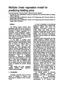
We have implemented the QEA for multiple-case outlier detection in multiple linear regression model using MATLAB programming on a PC. We have arbitrarily used MAX_GEN = 500 and the population sizes (the numbers of individuals in the populations) have been chosen depending on the problem. For each dataset, the QEA has been arbitrarily run 100 times with different seeds for the random number generator and for all datasets the same set of seeds has been used. We have experimented with 10 well-referred datasets from [19, 21] – six datasets have one predictor variable, one dataset has two predictor variables, one dataset has three predictor variables, one dataset has four predictor variables, and one dataset has six predictor variables. We discuss here experimental result of each dataset separately. The first dataset that we have experimented with is the Hertzsprung-Russel diagram of the CYG OB1 star cluster from [21], which is an often analyzed dataset in statistical literatures. The data is taken from 47 stars in the direction of Cygnus. The independent predictor variable is the log of the effective temperature at the surface of each star and the dependent response variable is the log of the star’s light intensity. We will refer to this dataset as CYG dataset. This dataset is analyzed by many researchers as an interesting masking problem. Figure 1 shows the scatter plot, least-squares (LS) lines with and without outliers, and LMS line for this dataset. Figure 1 shows that four data points 11, 20, 30, and 34 are clearly apart from the bulk. Two other data points 7 and 9 follow the same direction as of the previous four. Four data points 11, 20, 30, and 34 are reported as outlier in [4, 21]. Five data points 7, 11, 20, 30, and 34 are reported as outlier in [22]. Six data points 7, 9, 11, 20, 30, and 34 are reported as outliers in [23]. For this dataset we have arbitrarily © 2010 ACADEMY PUBLISHER

34 30

6.0

IV. EXPERIMENTAL RESULTS

20 11 9

5.5

•

LS line 5.0

•

For a given dataset, run the QEA a number of times with different seeds for the random number generator for different runs, so that the random number generator generates different sequences of random numbers in different runs and the different runs follow different search paths. For each run of the QEA, use a range of K values from under penalty (a K value that detects a set of outliers with cardinality ⎣N 2⎦ 100% of times or K = 1 ) to over penalty (a K value that detects no outliers 100% of times). Select the set of outliers that is detected by most K values. Break the tie by selecting the set of outliers that is detected most of the times.

Log light intensity

•

7 4.5

For a given dataset, the proposed QEA is run several times with different K values and the potential set of outliers is determined using the following technique:

LS line without outlier

LMS line

4.0

Step (x): The binary solution z among Z (t ) and b having the lowest f ( z ) value is stored into b .

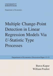
used population size 100. The “number of outliers detected” versus “% of times outlier detected” for this dataset is shown in Figure 2. From Figure 2, we see that seven outliers are detected 2% of times, 15 outliers are detected 3% of times, and 23 outliers are detected 95% of times by K = 1 . As 23 is exactly equal to ⎣N 2⎦ = ⎣47 2⎦ , we have not considered this set as potential outlier set, since the cardinality of the potential outlier set is less than ⎣N 2⎦ . We will use the same argument in the following experiments also. Six outliers are detected 93% of times by K = 2 . Four outliers are detected 18% of times by K = 3 . Each potential outlier set is detected by only one K value, but the outlier set with six outliers is detected highest percentage of times (93% of times) by K = 2 . Therefore, we have selected outlier set with six outliers (data points 7, 9, 11, 20, 30, and 34) as potential outliers for this dataset, which is also reported as outliers in [23]. However, data points 7 and 9 are not detected as outliers in [4, 21] and data point 9 is not detected as outlier in [22] due to smearing and/or masking, but our QEA can detect them as outliers. This implies that our QEA overcomes the effects of smearing and masking. From Figure 1, we also see that the LS line for 41 data points without the six detected outliers (data points 7, 9, 11, 20, 30, and 34) and the LMS line of all 47 data points are in the same direction. The second dataset we have experimented with is the Kootenary River Data from [21, 24], which has 13 data points. These data are measurements of water flow at two

3.6

3.8

4.0

4.2

4.4

4.6

Log temperature

Figure 1. Scatter plot, LS line with and without outliers, and LMS line for CYG Data. 100 90 80 % of times detected

rotation angle for our experiments. Readers can see [13] for more details of updating Q-bit individuals.

1783

70

k=1

60

k=2

50

k=3

40

k=4

30 20 10 0 0

2

4

6

10 12 14 16 8 No. of outlier detected

18

20

Figure 2. Outlier set identification in CYG Data.

22

JOURNAL OF COMPUTERS, VOL. 5, NO. 12, DECEMBER 2010

20

20

30

1784

LMS line

19 18

15

LS line without outlier

LS line

16 15

10

Phone calls

25

Newgate

17

5

20

LS line

21 LS line without outlier LMS line

0

4

20

30

40

50

60

50

70

55

60

Figure 3. Scatter plot, LS line with and without outlier, and LMS line for Kootenary River Data.

70

Figure 5. Scatter plot, LS line with and without outliers, and LMS line for Belgium Data.

100

100

90

90 % of times outlier detected

k=4

80 % of times detected

65 Year

Libby

70

k=2

60

k=3-14

50

k=15

40 30 20

k=5

80

k=6

70

k=7

60

k=8 k=9

50

k=10

40

k=11

30

k=12

20

k=13 k=14

10

10

k=15

0

0

0

0

1

2 3 4 No. of outlier detected

5

6

Figure 4. Outlier set identification in Kootenary River Data.

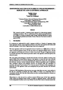
different points (Libby and Newgate) on the Kootenary River in January for the years 1931 to 1943. The independent predictor variable is the water flow at Libby point and the dependant response variable is water flow at Newgate point. Figure 3 shows the scatter plot, LS lines with and without outlier, and LMS line for this dataset. Data point 4 is reported as outlier in [21]. For this dataset we have arbitrarily used population size 100. The “number of outliers detected” versus “% of times outlier detected” for this dataset is shown in Figure 4. From Figure 4, we see that one outlier (data point 4) is detected 100% of times by K = 3,4, L ,14 , which is also reported as outlier in [21]. Therefore, our QEA successfully detects the only known outlier. From Figure 3, we also see that the LS line for 12 data points without the one detected outlier (data point 4) and the LMS line of all 13 data points are in the same direction. The third dataset we have experimented with is the Belgium dataset from [21], which has 24 data points and shows the number of international phone calls (in tens of millions) from Belgium during 1950 to 1973. For this dataset, the last two digits of the year is the independent predictor variable and the number of calls is the dependent response variable. Figure 5 shows the scatter plot, LS lines with and without outliers, and LMS line for this dataset. Figure 5 shows that this time series data contains heavy contamination for data points 15 to 20 (years 1964 to 1969). These data points are reported as

© 2010 ACADEMY PUBLISHER

1

2

3

4 5 6 7 8 No. of outlier detected

9

10

11

12

Figure 6. Outlier set identification in Belgium Data.

outliers in [4, 21]. For this dataset we have arbitrarily used population size 100. The “number of outliers detected” versus “% of times outlier detected” for this dataset is shown in Figure 6. From Figure 6, we see that seven outliers are detected by six different K values ( K = 9,10,11,12,13,14 ) and eight outliers are detected by four different K values ( K = 5,6,7,8) . As outlier set with seven outliers (data points 15, 16, 17, 18, 19, 20, and 21) is detected by most K values (six K values), we have selected this set as potential outliers in this data set. Six data points (data points 15, 16, 17, 18, 19, 20) are reported as outliers in [4, 21] and are detected by our QEA. Moreover, data point 21 is also detected as outlier by our QEA. To test whether the data point 21 is a 2 potential outlier, we have calculated e21 = 2.310 ; standard deviation of ei2 s, sd = 0.193 ; mean of ei2 s, e 2 = 0.172 ; and e 2 + 3sd = 0.751 for 18 data points (excluding data points 15, 16, 17, 18, 19, and 20), which shows that the square of the residual for the data point 21 lies outside the normal distribution of the squares of the residuals. Therefore, the data point 21 is a potential outlier, which is detected by our QEA. However, the sequential outlier detection method could not detect this data point as outlier due to smearing and/or masking. From Figure 5, we also see that the LS line for 17 data points (excluding the detected outlier points 15, 16, 17, 18, 19, 20, and 21) and the LMS line of all 24 data points

1785

120

JOURNAL OF COMPUTERS, VOL. 5, NO. 12, DECEMBER 2010

LS line LMS line

90

Gesell Adaptive Score

100

300

LS line without outlier

8

0

LS line without outlier & LMS

60

70

80

200

LS line

100

Growth of Price

19

110

9

40

42

44

46

10

48

20

Figure 7. Scatter plot, LS line with and without outliers, and LMS line for China Data. 100

% of times detected

80 70 60 50 40 30 20 10 0 0

1

2 No. of outlier detected

40

3

Figure 9. Scatter plot, LS line with and without outlier, and LMS line for Gesell Adaptive Score Data. 100 90 80 70 60 50 40 30 20 10 0

% of times detected

k=11 k=12 to 25 k=26 to 28 k=29

90

30

Age at First word (Month)

Year

4

Figure 8. Outlier set identification in China Data.

k=1 k=2 k=3 k=4

0

1

2

3 4 5 6 7 No. of outlier detected

8

9

10

Figure 10. Outlier set identification in Gesell Adaptive Score Data.

are the same, which is also in favor of the conclusion that data point 21 is a potential outlier. The fourth dataset we have experimented with is the China dataset from [21], which is a record of the annual rates of growth of average prices in the main free cities of free China from 1940 to 1948. The dataset has nine data points. The independent predictor variable is the last two digits of the year and the dependent response variable is the growth of price. Figure 7 shows the scatter plot, LS lines with and without outliers, and LMS line for this dataset. The data points 8 and 9 are reported as outliers in [4, 21]. For this dataset we have arbitrarily used population size 100. The “number of outliers detected” versus “% of times outlier detected” for this dataset is shown in Figure 8. From Figure 8, we see that two outliers are detected 100% of times by 14 different K values ( K = 12, L ,25 ), and one outlier is detected 100% of times by three different K values ( K = 26,27,28 ). As outlier set with two outliers (data points 8 and 9) is detected by most K values (14 different K values), we have selected this set as potential outliers in this data set. Thus, our QEA successfully detects all known outliers for this data set. From Figure 7, we see that the LS line for seven data points (excluding the detected outlier points 8 and 9) and the LMS line of all nine data points are the same. The fifth dataset we have experimented with is the Gesell Adaptive Score dataset from [21]. The dataset has 21 data points. The independent predictor variable is the

© 2010 ACADEMY PUBLISHER

age (in months) at which a children utters its first words and the dependent response variable is its Gesell adaptive score. Figure 9 shows the scatter plot, LS lines with and without outlier, and LMS line for this dataset. The data point 19 is reported as outliers in [21, 25]. For this dataset we have arbitrarily used population size 100. The “number of outliers detected” versus “% of times outlier detected” for this dataset is shown in Figure 10. From Figure 10, we see that one outlier (data point 19) is detected 5% of times by K = 2 and the same outlier is detected 100% of times by K = 3 . Therefore, we have selected data point 19 as potential outlier in this data set. Thus, our QEA successfully detected the only known outlier for this data set. From Figure 9, we see that the LS line for 20 data points (excluding the detected outlier data point 19) and the LMS line of all 21 data points are in the same direction. The sixth dataset we have experimented with is the Brain dataset from [21], which contrasts body weight (in kilograms) against the brain weight (in grams) of 28 different animal species. The independent predictor variable is the body weight and the dependent response variable is the brain weight. Figure 11 shows the scatter plot, LS lines with and without outliers, and LMS line for this dataset. The data points 6, 16, and 25 are reported as outliers in [4, 21]. For this dataset we have arbitrarily used population size 100. The “number of outliers detected” versus “% of times outlier detected” for this

1786

JOURNAL OF COMPUTERS, VOL. 5, NO. 12, DECEMBER 2010

dataset is shown in Figure 12. From Figure 12, we see that two outliers are detected by seven different K values ( K = 7, L ,13 ), three outliers are detected by two different K values ( K = 5,6 ), five outliers are detected by nine different K values ( K = 5, L ,13 ), six outliers are detected by one K value ( K = 4 ), seven outliers are detected by one K value ( K = 3 ), and 11 outliers are detected by three different K values ( K = 4,5,6 ). The outlier set with five outliers (data points 6, 7, 14, 16, 25) is detected by most (nine) K values and we have taken this outlier set as potential outlier set. The three data points 6, 16, and 25 are reported as outliers in [4, 21] and are also detected by our QEA. Besides these three known outliers, our QEA has detected two more data points (data points 7 and 14) as outliers. To test whether the data points 7 and 17 are potential outliers, we have calculated 2 e72 = 4038227.59 ; e14 = 1145544.56 ; standard deviation of ei2 s, sd = 270894.4 ; mean of ei2 s, e 2 = 249222.82 ; and e 2 + 3sd = 1061906.02 for 25 data points (excluding data points 6, 16, and 25), which shows that the square of the residual for the data points 7 and 14 lie outside the normal distribution of the squares of the residuals. Therefore, the data points 7 and 14 are potential outliers, which are detected by our QEA. However, the sequential outlier detection method could not detect these data points as outliers due to smearing and/or masking. This

and masking. From Figure 11, we also see that the LS line for 23 data points without the five detected outliers (data points 6, 7, 14, 16, and 25) and the LMS line of all 28 data points are in the same direction. The seventh dataset we have experimented with is the Aircraft dataset from [21], which has 23 data points. The four independent predictor variables are aspect ratio, liftto-drag ratio, weight of the aircraft (in pound), and the maximum thrust. The dependent response variable is the cost. As the dimension of the data set is five, we cannot draw the scatter plot, LS lines with and without outliers, and LMS line for this dataset. However, the data points 16 and 22 are reported as outliers in [26]. For this dataset we have arbitrarily used population size 5. The “number of outliers detected” versus “% of times outlier detected” for this dataset is shown in Figure 13. From Figure 13, we see that one outlier is detected by one K value ( K = 5 ), and two outliers are detected by three K values ( K = 2,3,4 ). The outlier set with two outliers (data points 16 and 22) is detected by most (three) K values and we have taken this outlier set as potential outlier set. Therefore, our QEA has successfully detected the known outlier set for this dataset. The eighth dataset we have experimented with is the Modified Wood Specific Gravity dataset from [21], which has 20 data points. The five independent predictor variables are anatomical factors and the dependent response variable is the wood specific gravity. As the dimension of the dataset is six, we cannot draw the scatter plot, LS lines with and without outliers, and LMS line for this dataset. However, the data points 4, 6, 8, and 19 are

5000

LMS line

100 7

% of times outlier detected

3000

LS line without outlier

2000

Brain Weight

4000

90

1000

14 LS line

80

k=1

70

k=2 k=3

60

k=4

50

k=5

40

k=6

30 20 10

0

16

6

25

0 0

0

20000

40000

60000

1

2

3

4 5 6 7 No. of outlier detected

80000

8

9

10

11

Body Weight

Figure 13. Outlier set identification in Aircraft Data. Figure 11. Scatter plot, LS line with and without outliers, and LMS line for Brain Data.

100

k=2 k=4 k=6 k=8 k=10 k=12 k=14

% of times outlier detected

90 80 70 60 50

k=3 k=5 k=7 k=9 k=11 k=13

40 30

% of times detected

100

90

k=2

80

k=3

70

k=4

60

k=5

50

k=6 k=7

40

k=8

30

k=9

20

20

k=10

10

10

0

0 0

1

2

3

4

5 6 7 8 9 No. of outlier detected

10

11

12

Figure 12. Outlier set identification in Brain Data.

implies that our QEA overcomes the effects of smearing

© 2010 ACADEMY PUBLISHER

0

1

2

3

4 5 6 7 No. of outlier detected

8

9

10

Figure 14. Outlier set identification in Modified Wood Specific Gravity Data.

JOURNAL OF COMPUTERS, VOL. 5, NO. 12, DECEMBER 2010

© 2010 ACADEMY PUBLISHER

100 % of times outlier detected

90 80 k=2

70

k=3

60

k=4

50

k=5

40

k=6

30

k=7

20 10 0 0

1

2

3

4 5 6 7 No. of outlier detected

8

9

10

Figure 15. Outlier set identification in Stackloss Data.

100

% of times detected

reported as outliers in [21]. For this dataset we have arbitrarily used population size 5. The “number of outliers detected” versus “% of times outlier detected” for this dataset is shown in Figure 14. From Figure 14, we see that one outlier is detected by one K value ( K = 6 ), four outliers are detected by six different K values ( K = 4, L ,9 ), six outliers are detected by one K value ( K = 6 ), and nine outliers are detected by two different K values ( K = 3,5 ). The outlier set with four outliers (data points 4, 6, 8, and 19) is detected by most (six) K values and we have taken this outlier set as potential outlier set. Therefore, our QEA has successfully detected the known outlier set for this dataset. The ninth dataset we have experimented with is the Stackloss dataset from [21], which has 21 data points that describe the operation of a plant for the oxidation of ammonia to nitric acid. The three independent predictor variables are rate of production, temperature, and acid concentration. The dependent response variable is the stackloss. As the dimension of the data set is four, we cannot draw the scatter plot, LS lines with and without outliers, and LMS line for this dataset. However, the data points 1, 3, 4, and 21 are reported as outliers in [21]. For this dataset we have arbitrarily used population size 5. The “number of outliers detected” versus “% of times outlier detected” for this dataset is shown in Figure 15. From Figure 15, we see that one outlier is detected 2% of times by K = 4 and 2% of times by K = 6 , two outliers are detected by one K value ( K = 3 ), four outliers are detected 24% of times by K = 4 and 13% of times by K = 5 , five outliers are detected by one K value ( K = 3 ), and eight outliers are detected by one K value ( K = 6 ). Though outlier sets with one outlier and four outliers are detected by two K values, the outlier set with four outliers is detected more times (37% of times) than outlier set with one outlier (4% of times). Therefore, we have taken outlier set with four outliers (data points 1, 3, 4, and 21) as potential outlier set. Thus, our QEA has successfully detected the known outlier set for this dataset. The tenth dataset we have experimented with is the Scottish Hills Races dataset from [19], which is a record of 35 races in Scotland in 1984. The two independent predictor variables are the distance (in miles) and the climb (in feet). The dependent response variable is the record time (in seconds). As the dimension of the data set is three, we cannot draw the scatter plot, LS lines with and without outliers, and LMS line for this dataset. However, the data points 7, 18, and 33 are reported as outliers in [2, 11, 19]. For this dataset we have arbitrarily used population size 100. The “number of outliers detected” versus “% of times outlier detected” for this dataset is shown in Figure 16. From Figure 16, we see that one outlier is detected by three different K values ( K = 8,9,10 ), two outliers are detected by two different K values ( K = 6,7 ), and three outliers are detected by four different K values ( K = 2,3,4,5 ). As the outlier set with three data points (data points 7, 18, 33) is detected by most (four) K values, we have taken this outlier set as

1787

90

k=1

80

k=2

70

k=3

60

k=4-5

50

k=6-7

40

k=8-10

30

k=11

20 10 0 0

1

2

3

4

5

6 7 8 9 10 11 12 13 14 15 16 17 No. of outlier detected

Figure 16. Outlier set identification in Scottish Hills Races Data.

the potential outlier set. Thus, our QEA has successfully detected the known outlier set for this dataset. V. CONCLUSIONS Quantum-inspired evolutionary algorithm (QEA) for multiple-case outlier detection in multiple linear regression model is presented here. Experimental results with 10 well-referred datasets with two to six independent predictor variables and one dependent response variable from statistical literature [19, 21] show that the proposed QEA has detected all outliers previously detected using sequential outlier detection methods. Moreover, for two datasets with one independent predictor variable (Belgium dataset and Brain dataset), the QEA also has detected some more potential outliers that were not detected by sequential outlier detection methods due to smearing and/or masking. From this observation, we can conclude that the proposed QEA is completely able to avoid the potential problems of smearing and masking. Multiple-case outlier detection is combinatorial in nature and requires testing of 2 N − N − 1 subsets of data points as potential outliers, where N is the number of data points. For this practical limitation, multiple-case outlier detection is not used for large datasets. The superb performance of QEA for multiple-case outlier detection in multiple linear regression model will allow us to handle this practical limitation of large dataset very effectively.

1788

JOURNAL OF COMPUTERS, VOL. 5, NO. 12, DECEMBER 2010

REFERENCES rd

[1] V. Barnett and T. Lewis, Outliers in Statistical Data, 3 ed. Chichester: John Wiley, 1994. [2] J. Tolvi, “Genetic algorithms for outlier detection and variable selection in linear regression models,” Soft Computing, vol. 8, pp. 527-533, 2004. [3] K.D. Crawford, R.L. Wainwright, and D.J. Vasicek, “Detecting multiple outliers in regression data using genetic algorithms,” in Proceedings of the 1995 ACM/SIGAPP Symposium on Applied Computing, Nashville, TN, USA, 26 – 28 February 1995, pp. 351 – 356. [4] K.D. Crawford and R.L. Wainwright, “Applying genetic algorithms to outlier detection,” in Proceedings of the 6th International Conference on Genetic Algorithms (ICGA95), Pittsburgh, PA, USA, L. Eshelman, Eds. Morgan Kaufmann Publisher, July 1995, pp. 546-550. [5] W. Cheney and D. Kincaid, Numerical Mathematics and Computing, Monterey: Brooks/Cole, 1980. [6] W.W. Hager, Applied Numerical Linear Algebra, Englewood Cliffs: Prentice Hall, 1988. [7] R.D. Cook and S. Weisberg, Residuals and Influence in Regression, London: Chapman and Hall, 1982. [8] D.F. Andrews and D. Pregibon, “Finding the outliers that matter,” Journal of the Royal Statistical Society B, vol. 40, pp. 85-93, 1978. [9] L. Davis, Handbook of Genetic Algorithms. New York: Van Nostrand Reinhold, 1991. [10] G. Schwarz, “Estimating the dimension of a model,” The Annals Stat, vol. 6, pp. 461-464, 1978. [11] O.G. Alma, S. Kurt, and A. Ugur, “Genetic algorithm based outlier detection using Bayesian information criterion in multiple regression models having multicollinearity problems,” G. U. Journal of Science, vol. 22, no. 3, pp. 141-148, 2009. [12] R.L. Mason, R.F. Gunst, and J.T. Webster, “Regression analysis and problems of multicollinearity,” Communication in Statistics, vol. 4, no. 3, pp. 277-292, 1975. [13] K.-H. Han and J.-H. Kim, “Quantum-inspired evolutionary algorithm for a class of combinatorial optimization,” IEEE Transactions on Evolutionary Computation, vol. 6, no. 6, pp. 580-593, Dec. 2002. [14] K.-H. Han and J.-H. Kim, “Quantum-inspired evolutionary algorithms with a new termination criterion, H∈ gate, and two-phase scheme,” IEEE Transactions on Evolutionary Computation, vol. 8, no. 2, pp. 156-169, April 2004.

© 2010 ACADEMY PUBLISHER

[15] K.-H. Kim, J.-Y. Hwang, K.-H. Han, J.-H. Kim, and K.-H. Park, “A quantum-inspired evolutionary computing algorithm for disk allocation method,” IEICE Transactions on Information and Systems, vol. E86-D, no. 3, pp. 645649, March 2003. [16] Y. Kim, J.-H. Kim, and K.H. Han, “Quantum-inspired multiobjective evolutionary algorithm for multiobjective 0/1 Knapsack problems,” in Proceedings of the 2006 IEEE Congress on Evolutionary Computation, July 2006, pp. 9151-9156. [17] J.-S. Jang, K.-H. Han and J.-H. Kim, “Face detection using quantum-inspired evolutionary algorithm,” in Proceedings of the 2004 IEEE Congress on Evolutionary Computation, June 2004, pp. 2100-2106. [18] M.H.A. Khan and S. Akter, “Multiple-case outlier detection in least-squares regression model using quantuminspired evolutionary algorithm,” in Proceedings of the 12th International Conference on Computer and Information Technology (ICCIT 2009), Dhaka, Bangladesh, 21-23 December 2009, pp. 7-12. [19] S. Chatterjee and A.S. Hadi, Regression Analysis by Examples, New York: Wiley, 2006. [20] P.J. Rousseeuw, “Least median of squares regression,” Journal of the American Statistical Association, vol. 79, pp. 871-880, 1984. [21] P.J. Rousseeuw and A.M. Leroy, Robust Regression & Outlier Detection, New York: John Wiley & Sons, 1987. [22] A.S. Hadi, A.H.M.R. Imon, and M. Werner, “Detection of outliers,” Computational Statistics, vol. 1, pp. 57-70, 2009. [23] A.A.M. Nurunnabi, Robust Diagnostic Deletion Techniques in Linear and Logistic Regression, MPhil Thesis, Department of Statistics, University of Rajshahi, Rajshahi, Bangladesh, 2008. [24] F.R. Hampel, E.M. Ronchetti, P.J. Rousseeuw, and W.A. Stashel, Robust Statistics: The Approach Based on Influence Function, New York: Wiley & Sons, 1986, [25] M.R. Mickey, O.J. Dunn, and V. Clark, “Note on the use of stepwise regression in detecting outliers,” Computational Biomedical Research, vol. 1, pp. 105-111, 1967. [26] A.H.M.R. Imon, “Identifying multiple influential observations in linear regression,” Journal of Applied Statistics, vol. 32, no. 9, pp. 929-946, 2005.