Output-Sensitive Algorithms for Optimally Constructing the Upper Envelope of Straight Line Segments in Parallel 1 N. Gupta a,∗, S. Chopra b , a Department
of Computer Science, University of Delhi, New Delhi 110007, India.
b Department
of Computer Science, New York University, New York, NY 10012, USA
Abstract The importance of the sensitivity of an algorithm to the output size of a problem is well known especially if the upper bound on the output size is known to be not too large. In this paper we focus on the problem of designing very fast parallel algorithms for constructing the upper envelope of straight-line segments that achieve the O(n log H) work-bound for input size n and output size H. When the output size is small, our algorithms run faster than the algorithms whose running times are sensitive only to the input size. Since the upper bound on the output size of the upper envelop problem is known to be small (nα(n)), where α(n) is a slowly growing inverse-Ackerman’s function, the algorithms are no worse in cost than the previous algorithms in the worst case of the output size. Our algorithms are designed for the arbitrary CRCW PRAM model. We first describe an O(log n·(log H+log log n)) time deterministic algorithm for the problem, that achieves O(n log H) work bound for H = Ω(log n). We then present a fast randomized algorithm that runs in expected time O(log H ·log log n) with high probability and does O(n log H) work. For log H = Ω(log log n), we can achieve the running time of O(log H) while simultaneously keeping the work optimal. We also present a fast randomized algorithm that runs in ˜ O(log n/ log k) time with nk processors, k > logΩ(1) n. The algorithms do not assume any prior input distribution and the running times hold with high probability. Key words: Parallel algorithm, Computational geometry, Upper envelope, Randomized algorithm
∗ Corresponding author. Tel. : +91-11-2766-7591; Fax: +91-11-2766-2553 Email addresses:
[email protected] (N. Gupta),
[email protected] (S. Chopra ). 1 A preliminary version of the paper appeared in twenty first annual symposium on FSTTCS
Preprint submitted to JPDC
11 January 2007
1
Introduction
The upper envelope of a set of n line segments in the plane is an important concept in visibility and motion planning problems. The segments are regarded as opaque obstacles, and their upper envelope consists of the portion of the segments visible from the point (0, +∞). The complexity of the upper envelope is the number of distinct pieces of segments that appear on it. If the segments are non-intersecting, then the complexity of their upper envelope is linear in n. On the other hand, if the segments are allowed to intersect, then the worst case complexity of the upper envelope increases to O(nα(n)), where α(n) is the functional inverse of Ackermann’s function [2]. A maximal appearance of a line segment s in the upper envelope is a maximal open interval (a, b) such that s appears on the envelope for all x in (a, b). Thus the complexity of the upper envelope is the total number of maximal appearances of all the line segments. We shall call a maximal appearance of a line segment in the upper envelope as an edge of the upper envelope. There exists an O(n log n) algorithm to compute the upper envelope of n line segments, and this is worst case optimal [23]. However this is true only if the output size, i.e., the number of vertices (or the edges) of the upper envelope is large. More specifically, the time-bound of O(n log n) is tight when the ordered output size is Ω(n). However if the output size is small then we should be able to do much better. For example consider the arrangement of the input line segments shown in figure 1. Clearly the complexity of the upper envelope (the output size) is a constant. In such situations an algorithm whose sequential running time is O(nH) (H being the output size), would runs faster than an O(nlogn) sequential time algorithm. The same argument carries to parallel algorithms as well. Thus the output-size of a problem is an important parameter in measuring the efficiency of an algorithm and one can get considerably superior algorithms in terms of it. There exists an O(n log H) algorithm for the problem [26], where H is the output size. This implies a linear time algorithm for constant output size. Thus, a parameter like the outputsize captures the complexity of the problem more accurately enabling us to design superior algorithms. The primary objective of designing parallel algorithms is to obtain very fast solutions to problems keeping the total work (the processor-time product) close to the best sequential algorithms. We are aiming at designing an output size sensitive parallel algorithm that speeds up optimally with output size in the sub-logarithmic time domain. We also present a sub-logarithmic time algorithm that uses super linear number of processors. The results have been obtained for arbitrary Concurrent Read Concurrent Write Parallel Random Access Machine (CRCW PRAM). 2
Fig. 1. An example of arrangement of line segments where the size of the upper envelope is constant. In such cases an algorithm whose running time depends on the output size H, for example O(n log H), will run in almost linear time.
1.1 Previous results
In the context of sequential algorithms, it has been observed that the upper envelope of n line segments can be computed in O(nα(n) log n) time, by a straight forward application of divide-and-conquer technique. Hershberger describes an optimal O(n log n) algorithm by reorganizing the divide-andconquer computation [23]. Clarkson describes a randomized O(nα(n) log n) algorithm for computing a face in an arrangement of line segments [11]. The upper envelope of line segments can be viewed as one such face. Guibas et al. [18], gave a deterministic algorithm which computed a face for a collection of line segments in O(nα2 (n) log n) time. The process of gift wrapping amounts to locating an extreme segment of the upper envelope and then “walking” along successive segments of the envelope which are defined by the points of intersection of the lines in the given arrangement. Thus if H is the size of the output, then it is easy to design an O(nH) time algorithm like the Jarvis’ March for convex hulls. There exists a deterministic sequential output sensitive algorithm due to Franck Nielsen and Mariette Yvinec that computes the upper envelope in O(n log H) time [26]. Their algorithm is based on the marriage-before-conquest paradigm to compute the convex hull of a set of fixed planar convex objects, which they also apply to compute the upper envelope of line segments. They use the partitioning technique of Hershberger to get an O(n log H) time for upper envelope. They claim that their algorithms are easily parallelizable onto EREW PRAM multi-computers following the algorithm of S. Akl [3]. This implies a parallel output sensitive algorithm which is optimal for number of processors bounded by O(nz ), 0 < z < 1. Dehne etal. in [14] have presented a parallel algorithm for the problem. Their n algorithm runs in O( n log +Ts (n, p)) time, where Ts (n, p) is the time for global p 3
sorting on p processors each with O( np ) local memory. Their bounds hold for √ small number of processors, i.e., for p ≤ n. Ts (n, p) depends upon a particular √ architecture. It is Θ( np (log n + p)) on a 2d-mesh, O( np (log n + log2 p)) on a n hypercube and O( n log ) on a fat-tree [14]. Since Ts (n, p) dominates for all the p architectures, √ it leads to an algorithm with√the same complexities as Ts (n, p). Since p ≤ n, the best time achievable is n log n on any architecture. In [5] Bertolotto etal. have also given a parallel algorithm with similar complexity. n + nα(n)) time. Here They also present an algorithm that runs in O( n log p also their algorithm is optimal only for a very small number of processors (when p < log n/α(n)) and the time taken is at least nα(n). Later Wei Chen and Koichi Wada gave a deterministic algorithm that computes the upper envelope of line segments in O(log n) time using O(n) processors [9]. If the line segments are non-intersecting and sorted, the envelope can be found in O(log n) time using O(n/ log n) processors. Their methods also imply a fast sequential result: the upper envelope of n sorted line segments can be found in O(n log log n) time, which improves the best-known bound O(n log n). A more detailed comparison of our algorithms with the others is given in the end.
1.2 Our algorithms and results We present algorithms whose running times are output-sensitive in the sublogarithmic time range while keeping the work (processor-time product) optimal [20]. For designing fast output-sensitive algorithms we have to cope with the problem that the output-size is an unknown parameter. Moreover we also have to rapidly eliminate input line segments that do not contribute to the final output without incurring a high cost. The two most successful approaches used in the sequential context, namely gift-wrapping and divide-and-conquer do not translate into fast parallel algorithms. By ‘fast’ we imply a time complexity of O(log H) or something very close. The gift-wrapping is inherently sequential taking O(H) sequential phases. Even the divide-and-conquer method is not particularly effective as it cannot divide the output evenly – in fact this aspect is the crux of the difficulty of designing fast output-sensitive algorithms that run in O(log H) time. We present one deterministic and two randomized algorithms that construct the upper envelope of n line segments. Both our randomized algorithms are of Las Vegas type. That is we always provide a correct output and the bounds hold with high probability. The term high probability implies probability exceeding 1-1/nc for any predetermined constant c and the input size n. We first describe a deterministic algorithm for the problem that takes O(log n· (log H + log log n)) time using O(n/ log n) processors. The algorithm is based on the ideas presented by Neilsen and Yvinec [26] to bound the size of the sub4
problems. Our algorithm achieves O(n log H) work bound for H = Ω(log n). Our algorithm is faster than the only parallel output sensitive algorithm (as claimed by Neilsen and Mariette) which is optimal for the number of processors bounded by O(nz ), 0 < z < 1. Next we present a fast randomized algorithm. The expected running times hold with high probability. The fastest algorithm runs in O(log H) expected time using n processors for H > logε n, and ε > 0. For smaller output sizes, the algorithm has an expected running time of O(log H · log log n) keeping the number of operations optimal. Therefore for small output sizes our algorithm runs very fast. Comparing this with (n, log n) algorithm of Chen and Wada [9], our algorithm is faster for small H. The algorithm uses the iterative method of Gupta and Sen [21]. We pickup a sample of constant size, filter out the redundant line segments and iterate, squaring the size of the sample at each iteration, until the size of the problem reduces to some threshold or the sample size increases to some threshold. We are able to achieve the bounds due to the Random Sampling Lemmas of Clarkson and Shor [12]. Next we describe a randomized algorithm that solves the problem in O(log n/ log k) time with high probability using super linear number of processors for k > logΩ(1) n. This algorithm is based on the general technique given by Sen to develop sub-logarithmic algorithms [34]. We finally compare the performance of our algorithm with other parallel algorithms both in terms of time complexity and work done. We are not aware of any previous work where the parallel algorithms for computing the upper envelope speed-up optimally with output size in the sub-logarithmic time domain. However it is claimed that using Chen and Wada’s algorithm [9] together with the filtering technique described by Clarkson and Shor [12], one can obtain fast output sensitive algorithms for the problem.
2
Deterministic algorithm for upper envelope
2.1 The Idea Our algorithm is based on the Marriage-before-conquest technique and it uses the ideas presented by Neilsen and Yvinec [26] to bound the size of the subproblems. Let S be the set of n line segments. Let its upper envelope be denoted by UE(S). If we know that there exists a partition ∪ki=1 Pi of S into k subsets such that each subset Pi , for i ∈ [1, k] is a set of x-separated line segments, then in the marriage-before-conquest procedure we can bound the size of the sub-problems by (n/2 + k). We transform the set S into a set 5
T of line segments partitioned into subsets, each subset consisting of a set of non-overlapping line segments, such that UE(S) = UE(T ). We now apply the marriage-before-conquest procedure on the set T . To compute the set T , we partition the set S using a partition tree and use the communication of J. Hershberger to make the number of line segments in T linear (i.e. to make the size of T linear). With a good estimate of k, we run the marriagebefore-conquest procedure on the set T (the number of stages of this procedure depends on k), and reduce the total size of the problem to n/log n, after which the problem is solved directly. We use an iterative technique to estimate the value of k.
2.2 The vertical decomposition Let Q be a subset of S. Through each vertex of the upper envelope of Q, we draw a line parallel to y-axis. These parallel lines induce a decomposition of the line segments of Q into smaller line segments, which we call the tiny line segments (see Figure 2). We only keep the tiny line segments that participate in the upper envelope.
Fig. 2. Tiny line segments formed after vertical decomposition of Q.
Note that the part of a line segment not contributing to the upper envelope of Q will not contribute to the final upper envelope. The tiny line segments are x-separated i.e. they are non-overlapping. The number of these tiny line segments is equal to the complexity of the upper envelope. Each tiny line segment is defined by a single line segment.
2.2.1 The partition tree To generate the set T from the set S, we group the line segments of the set S into k groups and compute the vertical decomposition of each group. Thus the tiny line segments formed in this decomposition form the set T , which is partitioned into k subsets, each consisting of non-overlapping segments. However such a grouping technique does not guarantee that the size of the set T i.e., the total number of such tiny line segments is linear. 6
We use the technique of J. Hershberger to group the line segments of S. The main idea is to create groups so that the size of the vertical decomposition of each group remains linear. Let p be an integer. We define x(q) as the abscissa of the point q. We first compute a partition tree of depth log p on the end points of the line segments as presented by Neilsen and Yvinec. Consider the 2n endpoints of the n line segments. Compute, by recursive application of an algorithm to compute the median, a partition P = {P1 , P2 , . . . , Pp } of the 2n endpoints so that each sheaf Pi has size 2n/p and the sheaves are x-ordered, (i.e., x(p) < x(q) for all p ∈ Pi and for all q ∈ Pi+1 ). We consider the following p − 1 reference abscissa and p x-ranges: • For each sheaf Pi , we associate the x-range Xi = {x(pi ) : pi ∈ Pi }. Note that all the x-ranges of the sheaves are disjoint. • Two successive sheaves Pi and Pi+1 are separated by a vertical line x = ai , where ai could be any value between the right most abscissa in sheaf Pi and the left most abscissa in the sheaf Pi+1 . We shall call ai as the reference abscissa between two consecutive x-ranges Xi and Xi+1 . We build an interval tree IT upon these p−1 reference abscissa and p x-ranges: each leaf of the interval tree corresponds to the x-range of a sheaf and each internal node to an abscissa separating the sheaves. Then, we allocate the n line segments according to the lowest common ancestor of their two endpoints. At this step, all the segments are located in two kinds of sets: (1) Those staying at a leaf of IT. This means that the abscissa of the end points of these line segments is included in the x-range of the sheaf. We say that these line segments are unclassified. (2) Those lying in an internal node of IT. The line segments whose lowest common ancestor of the abscissa of their endpoints is the node corresponding to the abscissa ai , cross the vertical line x = ai . Following the communication of J. Hershberger [23], their upper envelope is linear in the number of line segments. He shows that the upper envelope of the segments allocated to a given internal node is linear because all these line segments cross a vertical line. We say that these segments are classified. We notice that the upper envelope of the line segments allocated to different nodes at the same internal level of IT is linear in the number of line segments By grouping the line segments of each internal level of the interval tree into ⌈ni /p⌉ groups, each of size p, and computing for each group the vertical decomposition of their upper envelope, we obtain an O(n/p+log p) groups. Thus P⌈log p⌉−2 we have a partition of the original set of n line segments into i=0 ⌈ni /p⌉ = O(n/p + log p) subsets each consisting of p x-separated line segments. We also group the unclassified line segments as follows: we pick up one segment from each leaf and form a group. There are at most n/p such groups, each of size 7
p. Thus we obtain a new set T , which is partitioned into O(2n/p + log p) subsets, each consisting of p x-separated tiny line segments, such that UE(T ) = UE(S). Thus a total of O((2n/p + log p) · p) tiny line segments are formed. To make the size of the set T linear, we choose p such that p log p < n. The partition tree can be constructed in O(log n · log p) time using n/ log n processors. Using (n, log n) algorithm of [9] to compute the upper envelope, the vertical decomposition in each group can be computed in O(log p) time with p processors or in O(log p · log n) time with p/ log n processors. We arrive at the following lemma. Lemma 1 For a fixed integer p such that p log p < n, the time taken to generate the set T partitioned into O(2n/p + log p) subsets each consisting of p x-separated line segments from the set S, such that UE(S) = UE(T) is O(log n · log p) using O(n/ log n) processors. Remark 2 Since median can be computed in constant time with high probability with n processors, we have a randomized algorithm to obtain the above partition in O(log p) time with n processors.
2.3 The Marriage-before-conquest procedure We assume that the partition ∪ki=1 Pi of the set T into k subsets such that each subset Pi , is a set of non-overlapping line segments, is given. Let |T | = cn. Find the median xm of the x− coordinates of the 2cn endpoints of the segments. Compute the edge b of the upper envelope intersecting the vertical line through xm . Delete the segments lying completely below b. Split the problem into two subproblems one consisiting of all those segments at least one of whose end points lie to the left of end point of b and the other consisiting of all those segments at least one of whose end points lie to the right of end point of b. Solve each subproblem recursively and merge the output together with the edge b. Since at most k segments (one from each partition) can intersect any vertical line, the size of the sub-problems is bounded by O(n/2 + k) , where k = O(2n/p + log p) = O(n/p), for p log p < n. Note 1 At every stage each sub-problem has at least one output edge.
2.3.1 The analysis Computing the median takes O(log n) time using n/ log n processors. The edge of the upper envelope intersecting the vertical line x = xm belongs to 8
the line segment whose intersection point with the line has the maximum ycoordinate. To find the two endpoints bounding the edge, we need to compute the intersection of the line segment (to which the edge belongs), with the rest of the line segments and find amongst them the two points lying immediately to the right and left of the vertical line x = xm . This can be done in O(log n) time using n/ log n processors. Thus at each stage of recursion O(log n) time is spent using n/ log n processors. Lemma 3 The size of the problem reduces to n/ log n after log H + log log n stages of the MBC procedure, which is ≤ log p if the integer p is such that H log n ≤ p . 2.4 The main algorithm We now present our main algorithm that computes the upper envelope of the set S of n line segments. The algorithm works in two phases: (1) The estimation phase : During this phase we find a good estimate of p such that p log p < n and after O(log p) stages of the MBC procedure, the size of the problem reduces to n/ log n. During the process, we also transform the set S of n line segments into the set T of O(n) line segments. (2) The terminating phase: During this phase we solve the problem (of size n/ log n) directly. Det-UE (1)a. p = c, where c is some constant (> 4). b. If p log p > n use an O(n, log n) algorithm to solve the problem directly and stop. c. Use the algorithm of Section 2.2.1. to form a set T of tiny line segments using p, from the set S. d. Use the MBC procedure on T for log p stages. e. Compute the total size of the sub-problems after this. If the size < n/log n, then goto Step 2, else square p and repeat. (2) Solve the problem directly using an O(n, log n) algorithm. From Lemma 3, the loop is guaranteed to terminate as soon as p > H log n. Hence p < (H log n)2 for all the iterations.
2.4.1 The analysis Let pe denote the estimate of p. Then pe < (H log n)2 . If pi is the ith estimation of p, then the total time spent in the estimation phase is 9
< O(log n ·
P
log pi )
= O(log n · log pe ) = O(log n · (log H + log log n)) The terminating phase takes additional O(log n) time. Thus we have the following theorem Theorem 4 The upper envelope of n line segments can be constructed in O(log n·(log H+log log n)) time using O(n/ log n) processors in a deterministic CRCW PRAM. Strictly speaking, we must add the time for processor allocation to this time. However that can also be done in the same bounds. Theorem 5 The upper envelope of n line segments can be constructed in H + log n · (log H + log log n)) time using p processors in a deterministic O( n log p CRCW PRAM.
Proof. Follows from Brent’s slow down lemma [7]. 2
3
The Randomized Output Sensitive Algorithm
In this section we present an output-size sensitive randomized algorithm using O(n) processors. Our algorithm is an iterative one. The underlying algorithm is similar to the algorithm described for the planar convex hulls by Gupta and Sen [21]. Hence the entire analysis of their algorithm goes through in our case also. However here we shall detail out the steps that are specific to our problem. We assume for simplicity that no more than two line segments intersect at the same point and the abscissa and ordinate of the end points of no two line segments and that of points of intersection are the same. We also include a line segment, say L at y = M, as one of our input, where M = min{yi } - ε, (ε > 0, 1 ≤ i ≤ n and yi = the minimum y-coordinate of the ith line segment). The x-coordinate of the left and the right end points of L are (min{xli } - ε) and (max{xri } + ε) respectively, (ε > 0, 1 ≤ i ≤ n and xli and xri are the left and the right x-coordinate respectively of the endpoints of the ith line segment). By the introduction of such a line segment the complexity of the upper envelope will at most double. Thus the upper envelope would look like as shown in Figure 3. 10
L:Y =M Fig. 3. The Upper Envelope after including the line segment L.
3.1 The Idea Let us denote the input set of straight line segments by S and their upper envelope by UE(S). The idea is to construct the upper envelope of a random sample R of line segments and filter out the redundant segments that do not contribute to UE(S). We pickup a sample of line segments of constant size, compute its upper envelope, discard all the redundant line segments and iterate on the reduced problem. In each successive iteration we square the size of the sample to be chosen. We iterate until either the size of the problem reduces to some threshold or the sample size becomes greater than some threshold. At this point, if the problem size reduces to less than nε , then we use a brute force algorithm to solve the problem in constant time, else we use the algorithm described by Chen and Wada [9] to compute the upper envelope directly. To prove any interesting result we must determine how quickly the problem size decreases. The Random Sampling Lemmas discussed in the next section guarantee that when a sample of size = Ω(H 2 ) is chosen, the problem size reduces fast.
3.2 The Random Sampling Lemmas For any subset P ⊆ S, consider an edge of the upper envelope of P . Draw two vertical lines, one through the left end point of this edge and the other through the right end point of this edge. We define a slab as the portion of the Euclidian plane E2 between these two vertical lines. A configuration σ (which we call region) is the region lying above the upper envelope in such a slab. No two such regions overlap. See Figure 4. We say that the line segments adjacent to σ define σ. Example in Figure 4 segments s1 , s2 , s3 define σ1 . Notice that we include the line segment L at y = M (defined previously) in 11
σ1 s3
s1
s2
Fig. 4. Regions formed by a subset of the set S. The defining line segments of the region σ1 are s1 , s2 , s3 .
every subset P of S. From now onwards, whenever we talk of a subset P of S we would actually be meaning P ∪ L. Let Π∗ (R) denote the set of regions induced by a random sample R and Πh (R) denote the set of critical regions i.e. the regions not containing any output vertex. The set of line segments intersecting a region σ is called the conflict list of σ and is denoted by L(σ) and its cardinality |L(σ)| denoted by l(σ) is called the conflict size. We will use the following results to bound the size of the reduced problem.
l1
l2
li
lrα(r)
Fig. 5. Regions belonging to the subspace Π∗ (R) of Π(R).
Lemma 6 [12,25]. For some suitable constant k and large n,
Pr
X
σ∈Π∗ (R)
l(σ) ≥ knα(r) ≤ 1/c ,
for some constant c > 1, where probability is taken over all possible choices of the random sample R. The above lemma gives a bound on the size of the union of the conflict lists. Lemma 7 [12,25]. For some suitable constant k1 and large n, 12
Pr
"
#
max l(σ) ≥ k1 (n/r) log r ≤ 1/c ,
σ∈Π∗ (R)
for some constant c > 1, where probability is taken over all possible choices of random sample R such that |R| = r. This lemma gives a bound on the maximum size of each sub-problem. A sample is “good” if it satisfies the properties of Lemmas 6 and 7 simultaneously. In fact, we have the following. Lemma 8 We can find a sample R which satisfies both Lemmas 6 and 7 simultaneously with high probability. Moreover, this can be done in O(log r) time and O(n log r) work with high probability. Proof. This can be done using Resampling and Polling technique of Reif and Sen [28]. See Appendix A for referrence. 2 Since |Πh (R)| ≤ H, a good sample clearly satisfies the following property also. Lemma 9 For a good sample R, P
σ∈Πh (R)
l(σ) = O(nH log r/r),
where |R| = r and Πh (R) is the set of all the regions that contain at least one output point. 3.3 The Algorithm We pick up a random sample R of S and compute its upper envelope. We will use this to delete the line segments which we know will not contribute to the final output and iterate. We say that a line segment is redundant if it does not intersect any critical region. That is, either it lies entirely below the upper envelope of R (see segment s1 in Figure 6) or it intersects some region lying above the upper envelope but not the critical region (segments s2 , s3 in figure 6). Consider a region that does not contain any output point. Clearly only one line segment is useful in this region, which is the line segment that has the maximum y-coordinate in that region. Such a line segment must intersect at least one of the regions containing an output point and is therefore retained. In Figure 6, the region Q2 does not contain any output point and the line segment L is the one with the maximum y-coordinate. Clearly L intersects 13
v1
v2
v3
s2 s3 s1 Q1
Q2
Q3
Q4
Q5
Q6
Q7 Q8
Q9
Fig. 6. Critical regions are Q1 , Q6 and Q8 . Non Critical regions are Q2 , Q3 , Q4 , Q5 and Q7 . The line segment L is retained because of regions Q1 and Q6 which contain output points namely v1 and v2 .
atleast one region containing an output point, namely Q1 and Q6 and hence is retained. Output points in these regions are v1 and v2 respectively. We delete the redundant line segments and iterate on the reduced problem. Lemma 9 will be used to estimate the non-redundant line segments whenever H ≤ r/ log r. Let Π∗ (R) denote the set of regions induced by a sample R (as defined in Section 3.2) and let ni (respectively ri ) denote the size of the problem (respectively sample size) at the ith iteration with n1 = n. Repeat the following procedure until ri > nε (this condition guarantees that the sample size is never too big) or ni < nε for some fixed ε between 0 and 1. If ni < nε , then find out the upper envelope of ni line segments directly using a brute force algorithm. Otherwise do one more iteration and find out ni+1 . If ni+1 = O(n1−ε/4), then we use a brute force algorithm, otherwise we use the algorithm of Chen and Wada [9] to find the upper envelope of ni+1 line segments. The following is the description of the ith iteration of the algorithm. Rand-UE (1) Use the procedure of Lemma 8. to choose a “good” sample R of size ri 2 for i > 1. = constant for i = 1 and ri−1 (2) Find out the upper envelope of R. (3) (a) For every line segment find out the slabs that it intersects. (b) Discard the redundant line segments lying below the upper envelope 14
of R. (Section 4 discusses this in detail). (c) If the sum taken over all the remaining line segments, of the number of regions intersecting a line segment is O(nα(r)) then continue else goto Step 1. (4) Filter out the segments not conflicting with any critical region as follows. (a) Compute Πh (R) as follows. For every region σ do the following: (i) Find out the line segments intersecting σ and assign l(σ)/α(r) processors to it (see Lemma 6. and Step 3(c) above). (ii) Consider the points of intersection of the line segments with the vertical lines defining the region (the boundaries of the slab lying above the edges of the upper envelope) including the intersection points by the edges of the upper envelope. If the points with maximum y-coordinate belong to the same line segment say s, and there does not exist any segment above s lying entirely in σ, then σ ∈ / Πh (R) else σ ∈ Πh (R). (b) Delete a line segment if it does not belong to ∪σ∈Πh (R) L(σ) (5) The set of line segments for the next iteration is ∪σ∈Πh (R) L(σ) and its size is ni+1 = | ∪σ∈Πh (R) L(σ)| Increment i and go to 1.
3.4 The Analysis
The analysis of Gupta and Sen [21] goes through here also. However detecting and deleting the redundant segments require further explanation which is done in Section 4. Assume that H = O(nδ ) for some δ between 0 and 1, for otherwise the problem can be solved in O(log n) = O(log H) time. Let n be the number of processors. Step 3(a) (finding the regions that a segment intersects) takes O(log ri ) time initially (when there is no processor advantage) until the sample size grows to Ω(H 2 ) (giving a geometric series with log H as the leading term) and constant time there onwards taking a total of O(log H + log log n) time, log log n being the total number of iterations. Steps 3(c), 4(a)(i) and 4(b) are implemented using procedures for Interval allocation, Processor allocation, Semisorting and Approximate compaction. These steps take O(α(r)+log∗ n) time initially until the size of the problem reduces to n/ log n (taking O(log∗ n log log log n) time, α(r) = O(α(n)) gets subsumed in O(log ∗n), log log log n being the number of iterations required to reduce the problem size to n/ log n), and constant time there onwards taking a total of O(log∗ n log log log n + log log n) time. Step 4(a)(ii) can be done in O(α(r)) time using n processors [21] until the size of the problem reduces to n/α(n) and constant time there onwards. Hence the 15
time for this step gets subsumed in that for the other steps. Let the terminating condition be satisfied in the tth iteration. If nt < nǫ , then computing the upper envelope of nt line segments takes constant time. Otherwise, if nǫ < rt < nt or nǫ < nt < rt then we have the following: Let ǫ be < 1/2. Clearly, rt−1 < nǫ and rt < n2ǫ . Hence we can afford to do one more iteration within the same bounds. Now, nt+1 = O(nt H log rt /rt ) = O(nt H(2ǫ log n)/nǫ ) = O(n1−ǫ/2 H). Now if nt+1 = O(n1−ǫ/4 ) the problem is solved directly in constant time using brute force method. Otherwise, we must have H = Ω(nǫ/4 ) and hence using the algorithm of Chen and Wada, the algorithm runs in O(log n) = O(log H) time. We thus arrive at the following lemma. Lemma 10 The upper envelope of n possibly intersecting straight line segments can be constructed in O(max{log H, log log n}) time with high probability using a linear number of processors, where H is the output size. Remark 11 For log H = Ω(log log n), this attains the ideal O(log H) running time with n processors, keeping the work optimal. Using n/ log log n processors instead of n and Brent’s Slow down Lemma, we have the following result Theorem 12 The upper envelope of n possibly intersecting straight line segments can be constructed in O(log H · log log n) expected time and O(n log H) operations with high probability in a CRCW PRAM model where H is the size of the upper envelope. Theorem 13 The upper envelope of n line segments can be constructed in H O( n log + log H · log log n) time using p processors in a deterministic CRCW p PRAM.
Proof. Follows from Brent’s slow down lemma [7]. 2
4
Finding the Redundant Line Segments
Recall that a segment is redundant if it does not intersect any critical region, i.e. either it lies entirely below the upper envelope of the random sample or it intersects some region lying above the upper envelope but not the critical region. For the purpose of this section, by the term redundant we mean the segments lying below the upper envelope of the sample. We develop a fast sublogarithmic algorithm that determines whether a line segment is redundant or 16
s1 v1 v5 v7
s6 R
e
d
u
n
d
a
n
N
o
n
t
v2
s5
R
s2
r2
r3
r5
r4
u
n
d
a
n
t
s3
s4 r1
d
v6
v4
v3
e
r6
r7
r8
Fig. 7. Segments s1 , s2 , s3 , s5 , s6 are Non Redundant. Segment s4 is Redundant.
not. The algorithm runs in O(log m/ log k) time using k processors, where m is the size of the upper envelope.
4.1 The idea
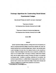
Consider an upper envelope of a random sample of line segments, divided into regions (as defined in Section 3.2). Consider any line segment (see Figure 7). If the line segment intersects the upper envelope at any point then it is nonredundant. However, if it does not intersect, then two cases arise: 1. Either the line segment lies entirely above the upper envelope in which case, it is non-redundant (segment s1 ). 2. The line segment lies entirely below the upper envelope (segment s4 ) in which case, it is redundant. So to determine if the line segment is redundant or not, we need to determine if it intersects the upper envelope. Let the vertices of the upper envelope spanned by a line segment be called the defining points for that line segment (for example v1 , v2 , . . . , v6 , v7 for line segment s6 ). If the line segment intersects the part of the envelope defined only by the defining points (segments s3 and s6 ), then the line segment intersects the upper envelope and hence, it is declared non-redundant. But if it does not intersect this part, then if the line segment lies above the upper envelope of its defining vertices, then it is non redundant. Else, if the line segment lies below the upper envelope of its defining vertices, we consider the two extreme slabs which the line segment intersects (for example s2 intersects the upper envelope in r7 and s5 in r2 ). If the line segment intersects the part of the envelope in these extreme slabs then it is non-redundant, else it is redundant. Thus the problem reduces to determining whether a line segment intersects part of the upper envelope defined by its defining vertices and whether it lies entirely below it, in case it does not. Then in additional constant time (checking the extreme slabs for intersection) we can determine whether the segment is redundant or not. The case when a line segment belongs entirely to one region is a special one in which the two extreme regions coincide. 17
Clearly, If a line segment intersects the lower convex chain of its defining vertices then it intersects the upper envelope defined by them. Note that the converse is not true.
v v2
v v1 Fig. 8. Any segment that intersects the lower convex chain of its defining vertices intersects it in two points, and it must intersect the upper envelope of these defining vertices.
Lemma 14 Given an upper envelope of size m, we can preprocess its vertices in constant time using O(m6 ) processors, such that given any arbitrary line segment with k processors, we can determine whether it is redundant or not in O(log m/ log k) time.
Proof. The lower convex chain for all the segments can be precomputed using a locus based approach in constant time using O(m6 ) processors. Given a line segment with k processors, we can perform k-way search for each of its end points in O(log m/ log k) time to find the vertices it spans. With k processors by a k-way search of the convex chain one can determine in O(log m/ log k) time whether the line segment intersects the convex chain and hence determine whether the segment is redundant or not. 2
5
˜ The O(log n/ log k) time algorithm
5.1 The Algorithm The general technique given by Sen [34] to develop sub-logarithmic algorithms can be used to design on O(log n/ log k) algorithm for the problem. Let the 18
number of line segments be n and the number of processors be (nk ), k > logΩ(1) n. (1) Pick up a good sample R of size (nk)1/c log n, for some suitable constant c > 1 which will be decided later. (2) Compute the upper envelope of the sample using a brute force algorithm. (3) Define the regions as explained in Section 3.2. (4) Determine the set of critical regions and remove all the redundant line segments as explained in Section 4. (5) If the size of the sub-problem is O(logΩ(1) n), then solve directly using a brute force algorithm else recurse. 5.2 The Analysis Assume the availabilty of nk processors. For c = 5, the sample size r is 1 (nk) 5 log n and the upper envelope of these segments can be computed in constant time using r 4 processors by a brute-force method. Critical regions are determined in O(log n/ log k) time as explained in Section 4 plus O(log n/ log k) time for semi-sorting. Deletion of redundant segments can be done by compaction using sorting. Thus if T (n, m) represents the parallel running time for the input size n with m processors then 1
1
T (n, nk) = T (n/(nk) c , nk/(nk) c ) + a log n/ log k
(1)
constants c and a are greater than 1. The solution of this recurrence with appropriate stopping criterion is O(log n/ log k) by induction. Hence we have the following. Theorem 15 Given n straight line segments and nk (k > logΩ(1) n) processors, we can find their upper envelope in O(log n/ log k) steps with high probability.
6
Comparison with Other Algorithms
In this section we compare the performance of our algorithm with others, both in terms of time complexity and the work done. The following table summarizes the relative results. One can clearly see from the table that our algorithms are work optimal in the output size and also very efficient in running time when the output size H is small. Our algorithms are designed for CRCW PRAM model. However, on 19
Algorithm
Procs.
Time
Work Done
Chen, Wada [9]
n
O(log n)
O(n log n)
Nielsen, Yvinec [26]
O(nz ) √ p≤ n
O(n1−z log H)
O(n log H)
n O( n log + Ts (n, p)) p
O(n log n + p.Ts (n, p))
n O( n log + nα(n)) p
O(n log n + pnα(n))
Dehne etal. [14] Bertolotto etal. [5] Bertolotto etal. [5] DET-UE
p √ p≤ n
O( logn n )
O( nα(n)p log n
+ Ts (n, p))
O(log n · (log H + log log n))
O(nα(n) log n + pTs (n, p)) O(n log H)
n RAND-UE O( log log O(log H · log log n) O(n log H) n) Table 1 Table giving the number of processors, time complexity and the work done by various algorithms. Ts (n, p) in the third and fifth rows is the time for global sorting on p processors each with O(n/p) memory [14,5]. It depends on the parallel architecture used.
any practical architecture, concurrent read and concurrent write operations can be simulated with communication graph of a complete binary tree of height log p. For example, a complete binary tree of height l can be embedded in a 2d-mesh with dilation ⌈ 2l ⌉ and in a hypercube of dimension l + 2 with dilation 1 [31]. With the direct application of the above facts, our algorithms can be implemented on a 2d-mesh by a slow down of at most log2 p and on a hypercube within the same bounds. Even with a slow down of log2 p on a 2d-mesh our algorithms are faster than the previous algorithms.
7
Remarks and Open Problems
First we presented a deterministic algorithm for the problem of upper envelope of line segments that runs in O(log n · (log H + log log n)) time and achieves O(n log H) work bound for H = Ω(log n). For small output sizes, we presented faster randomized algorithms for the problem. The fastest algorithm runs in O(log H) time using linear number of processors for a large range of output size, namely H ≥ logε n. For small output size our algorithm runs in O(log log n · log H) time and speeds up optimally with the output size. Finally we described a sub-logarithmic time parallel algorithm that runs in ˜ O(log n/ log k) time using nk processors, k > logΩ(1) n. One of the issues that remains to be dealt with is that of speeding up the algorithm further using a superlinear number of processors such that the time taken is Ω(log H/ log k) with nk processors, where k > 1. Designing an algorithm that takes O(log H) time and does optimal work for all values of H is another open problem. 20
The other issue is that of designing a sub-logarithmic time algorithm using superlinear number of processors for k > 1. This could be achieved if we are able to filter the redundant line segments to further restrict the blow up in problem size in successive levels of recursion and to allocate processors such that, to each sub-problem the number of processors allocated is bounded by its output size. The technique of Sen [28,34] to filter the redundant line segments and the processor allocation scheme used by them is not particularly effective here. According to that scheme, the number of processors which we must allocate to a segment is the number of vertices contributed by the segment to the output which we don’t know in advance in this case and moreover the requirement of a segment as it goes down the levels of recursion may increase. Appendix A Since the events of Lemmas 6 and 7 would fail only with constant probability, the probability that the conditions would fail in O(log n) independent trials is less than 1/nα for some α > 0. So we select O(log2 n) independent samples. One of them is “good” with high probability. However, to determine if a sample is “good” we will have to do step 3(a)i log2 n times each of which will take O(log r) time (we will show later). We can not afford to do this. Instead, we try to estimate the number of half-planes intersecting a region using only a fraction of the input half-planes. Consider a sample Q. Check it against a randomly chosen sample of size n/ log3 n of the input half-planes for the condition of Lemmas 6 and 7. We explain below how to check for these conditions. Our procedure works for r = o(n/ log4 n). For every region ∆ defined by Q do in parallel. Let A(∆) be the number of half-planes of the n/ log3 n sampled half-planes intersecting with ∆ and let X(∆) be the total number of half-planes intersecting with ∆. Let X(∆) > c′ log4 n for some constant c′ - the conditions of Lemmas 6 and 7 hold trivially for the other case (for r < cn/ log4 n for some constant c, (n log r)/r > n/r > (1/c) log4 n > (1/cc′ )X(∆) and P 4 ′ ′ ∆ X(∆) ≤ c r log n < c cn).
By using Chernoff’s bounds for binomial random variables, L = k1 ( ∆ A(∆) log3 n) P and U = k2 ( ∆ A(∆) log3 n) are lower and upper bounds respectively for P X = ∆ X(∆) with high probability, for some constants k1 and k2 . P
For some constant k,
(1) Reject a sample if L > kn (X ≥ L > kn). (2) Accept a sample if U ≤ kn (X ≤ U ≤ kn). (3) If L ≤ kn ≤ U then accept a sample. ( X/kn ≤ U/L, which is a constant).
21
With high probability about log n samples will be accepted by the above P procedure. Also clearly, ∆ A(∆) ≤ kn/ log3 n. For each of the samples accepted by the above proedure consider in parallel:
Again by using Chernoff’s bounds for binomial random variables, L(∆) = k1′ (A(∆) log3 n) and U(∆) = k2′ (A(∆) log3 n) are lower and upper bounds respectively for X(∆) with high probability, for some constants k1′ and k2′ . Each region reports whether to “accept” or to “reject” a sample as follows. For some constant k ′ , (1) Reject a sample if L(∆) > k ′ (n/r) log r (X(∆) ≥ L(∆) > k ′ (n/r) log r). (2) Accept a sample if U(∆) ≤ k ′ (n/r) log r (X(∆) ≤ U(∆) ≤ k ′ (n/r) log r). (3) If L(∆) ≤ k ′ (n/r) log r ≤ U(∆) then accept a sample. ( X(∆)/k ′ (n/r) log r ≤ U(∆)/L(∆), which is a constant) If any region reports “reject” a sample then reject the sample.
References [1] A. Agarwal, B. Chazelle, L. Guibas, C. O’Dunlaing and C. K. Yap, Parallel computational geometry. Proc. 25th Annual Sympos. Found. Comput. Sci. (1985) 468-477; also: Algorithmica 3 (3) (1988) 293-327. [2] P. K. Aggarwal and M. Sharir, Davenport-Schinzel Sequences and their Geometric Applications. (1995). [3] S. Akl, Optimal algorithms for computing convex hulls and sorting, Computing 33 (1) (1984) 1-11. [4] H. Bast and T. Hagerup, Fast parallel space allocation, estimation and integer sorting, Technical Report MPI-I-93-123 (June 1993). [5] M. Bertolotto, L. Campora, and G. Dodero. A Scalable Parallel Algorithm for Computing the Upper Envelope of Segments. Proceedings of Euromicro (1995), 503-509. [6] B. K. Bhattacharya and S. Sen, On simple, practical, optimal, output-sensitive randomized planar convex hull algorithm, J. Algorithms 25 (1997) 177-193. [7] R. Brent, Parallel evaluation of general arithmetic expressions, Journal of the ACM, (1974), 21, 201–206. [8] B. Chazelle and J. Friedman, A deterministic view of random sampling and its use in geometry, Combinatorica 10 (3) (1990) 229-249.
22
[9] W. Chen and K. Wada, On Computing the Upper Envelope of Segments in Parallel, Proceeding of 27th International Conference on Parallel Processing (1998), 253-260. [10] D. Z. Chen, W. Chen, K. Wada, K. Kawaguchi Parallel Algorithms for Partitioning Sorted Sets and Related Problems, Algorithmica 28, (2000), 217241. [11] K. L. Clarkson, A randomized algorithm for computing a face in an arrangement of line segments. [12] K. L. Clarkson and P. W. Shor, Applications of random sampling in computational geometry, II, Discrete Comput. Geom. 4 (1989) 387-421. [13] R. Cole, An optimal efficient selection algorithm, Inform. Process. Lett. 26 (1987/1988) 295-299. [14] F. Dehne, A. Fabri and A. Rau-Chaplin, Scalable Parallel Geometric Algorithms for Computing the Upper Envelope of Segments. Proceedings of 9th Annual ACM Symposium on Computational Geometry, (1993), 298 - 307. [15] H. Edelsbrunner, Algorithms in Combinatorial Geometry (Springer, New York, 1987). [16] P. B. Gibbons, Y. Matias, and V. Ramachandran, Efficient Low-Contention Parallel Algorithm. Proceedings of the 6th Annual ACM Symposium on Parallel Algorithms and Architectures, (1994), 236 - 247. [17] M. Goodrich, Geometric partitioning made easier, even in parallel, Proc. 9th ACM Sympos. Comput. Geom. (1993) 73-82. [18] L. J. Guibas, M. Sharir, and S. Sifrony, On the general motion planning problem with two degrees of freedom, Discrete Comput. Geom. , 4 (1989), 491-521 [19] N. Gupta, Efficient Parallel Output-Size Sensitive Algorithms, Ph.D. Thesis, Department of Computer Science and Engineering, Indian Institute of Technology, Delhi (1998). [20] N. Gupta, S. Chopra and S. Sen, Optimal, Output-Sensitive Algorithms for Constructing Upper Envelope of Line Segments in Parallel, Foundations of Software Technology and Theoretical Computer Science (Foundations of Software Technology and Theoretical Computer Science) , (2001) 183-194. [21] N. Gupta and S. Sen, Optimal, output-sensitive algorithms for constructing planar hulls in parallel, Comput. Geom. Theory and App. 8 (1997) 151-166. [22] N. Gupta and S. Sen, Faster output-sensitive parallel convex hull for d ≤ 3: optimal sub-logarithmic algorithms for small outputs, Proc. ACM Sympos. Comput. Geom. (1996) 176-185. [23] J. Hershberger, Finding the upper envelope of n line segments in O(n log n) time, Inform. Process. Lett. 33 (1989) 169-174.
23
[24] Fast and Scalable Paralle Matric Computations on Distributed Memory Systems. Proceedings of IPDPS 2005, IEEE (2005). [25] K. Mulmuley, Computational Geometry: An Introduction through Randomized Algorithms.(Prentice Hall, Englewood Cliffs, NJ, 1994). [26] F. Nielsen and M. Yvinec, An output-sensitive convex hull algorithm for convex objects. (1995). [27] F. P. Preparata and M. I. Shamos, Computational Geometry: An Introduction (Springer, New York, 1985). [28] S. Rajasekaran and S. Sen, in: J. H. Reif, Ed., Random Sampling Techniques and Parallel Algorithm Design (Morgan Kaufmann Publishers, San Mateo, CA, 1993). [29] E. A. Ramos, Construction of 1-d lower envelopes and applications, Proceedings of the thirteenth annual symposium on Computational geometry, (1997), 57-66. [30] T. Hagerup and R. Raman, Waste makes haste : tight bounds for loose parallel sorting, FOCS, 33, 1992, 628 – 637. [31] M. J. Quinn, Parallel Computing: Theory and Practice, McGraw-Hill, INC. [32] J. H. Reif and S. Sen, Randomized algorithms for binary search and Load Balancing on fixed connection networks with geometric applications, SIAM J. Comput. 23 (3) (1994) 633-651. [33] J. H. Reif and S. Sen, Optimal Parallel Randomized Algorithms for 3-D Convex Hull, and Related Problems, SIAM J. Comput. 21 (1992) 466-485. [34] S. Sen, Lower bounds for parallel algebraic decision trees, parallel complexity of convex hulls and related problems, Theoretical Computer Science. 188 (1997) 59-78.
24