Selection: The Harder You Try the Worse it Gets*. John Loughrey, Pádraig Cunningham. Trinity College Dublin, College Green, Dublin 2, Ireland. {John.
Overfitting in Wrapper-Based Feature Subset Selection: The Harder You Try the Worse it Gets
*
John Loughrey, Pádraig Cunningham Trinity College Dublin, College Green, Dublin 2, Ireland. {John.Loughrey, Padraig.Cunningham}@cs.tcd.ie
Abstract. In Wrapper based feature selection, the more states that are visited during the search phase of the algorithm the greater the likelihood of finding a feature subset that has a high internal accuracy while generalizing poorly. When this occurs, we say that the algorithm has overfitted to the training data. We outline a set of experiments to show this and we introduce a modified genetic algorithm to address this overfitting problem by stopping the search before overfitting occurs. This new algorithm called GAWES (Genetic Algorithm With Early Stopping) reduces the level of overfitting and yields feature subsets that have a better generalization accuracy.
1
Introduction
The benefits of wrapper-based techniques for feature selection are well established [1, 15]. However, it has recently been recognized that wrapper-based techniques have the potential to overfit the training data [2]. That is, feature subsets that perform well on the training data may not perform as well on data not used in the training process. Furthermore, the extent of the overfitting is related to the depth of the search. Reunanen [2] shows that, whereas Sequential Forward Floating Selection (SFFS) beats Sequential Forward Selection on the data used in the training process, the reverse is true on hold-out data. He argues that this is because SFFS is a more intensive search process i.e. it explores more states. In this paper we present further evidence of this and explore the use of the number of states explored in the search as an indicator of the depth of the search and thus as a predictor of overfitting. Clearly this metric does not tell the whole story since for example a lengthy random search will not overfit at all. We also explore a solution to this overfitting problem. Techniques from Machine Learning research for tackling overfitting include: − Post-Pruning: Overfitting can be eliminated by pruning as is done in the construction of Decision Trees [6].
*
This research was funded by Science Foundation Ireland Grant No. SFI-02 IN.1I111
− Jitter: Adding noise to the training data can make it more difficult for the learning algorithm to fit the training data and thus overfitting is avoided [12]. − Early Stopping: Overfitting is avoided in the training of supervised Neural Networks by stopping the training when performance on a validation set starts to deteriorate [7, 14]. Of these three options, the one that we explore here is Early Stopping. We present a stochastic search process that has a cross-validation stage to determine when overfitting occurs. Then the final search uses all the data to guide the search and stops at this point determined by the cross-validation. We show that this method works well in reducing the overfitting associated with feature selection – this will be shown later in Section 4. In Section 2 of the paper we briefly discuss different approaches to Feature Selection, focusing on various wrapper based search strategies. Section 3 provides more detail on the GAWES algorithm and early stopping in stochastic search. Section 4 outlines the results of the experimental study. Future avenues for research are discussed in Section 5 and the paper concludes in Section 6.
2
Wrapper-Based Feature Subset Selection
Feature selection is defined as the selection of a subset of features to describe a phenomenon from a larger set that may contain irrelevant or redundant features. Improving classifier performance and accuracy are usually the motivating factors behind this, as the accuracy is degraded by the presence of these irrelevant features. The curse of dimensionality is the term given to the phenomenon when there are too many features in the model and not enough instances to completely describe the target concept. Feature selection attempts to identify and eliminate unnecessary features, thereby reducing the dimensionality of the data, and hopefully resulting in an increase in accuracy. The two common approaches to feature selection are the use of filters and the wrapper method. Filtering techniques attempt to identify features that are related to or predictive of the outcome of interest: they operate independently of the learning algorithm. An example is Information Gain, which was originally introduced to Machine Learning research by Quinlan as a criterion for building concise decision trees [6] but it is now widely used for feature selection in general. The wrapper approach differs in that it evaluates subsets based upon the accuracy estimates provided by a classifier built with that feature subset. Thus wrappers are much more computationally expensive that filters but can produce better results because they take the bias of the classifier into account and evaluate features in context. A detailed presentation of the wrapper approach can be found in [1].
2.1 Search Algorithms The wrapper method can be viewed as a search optimization process and therefore can incur a high computational cost. From n features, the number of possible feature subsets is 2n, so it is impractical to search the whole state space except in situations
with a small number of features. The search strategies available can be classed into three categories; randomized, sequential and exhaustive, depending on the order in which they evaluate the subsets. In this research we only experiment with randomized and sequential techniques as an exhaustive search is infeasible in most domains. The algorithms we use are forward selection, backward elimination, hill climbing and a genetic algorithm as these tend to be quite popular and are easily implemented strategies.
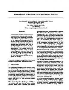
2.2 The Problem of Overfitting A classifier is said to overfit to a dataset if it models the training data too closely and gives poor predictions on new data. This occurs when there is insufficient data to train the classifier and the data does not fully cover the concept being learned. Such models are said to have a high variance, meaning that small changes in this data will have a significant influence on the resulting model [8]. This is a problem for many real world situations where the data available may be quite noisy. Overfitting in feature selection appears to be exacerbated by the intensity of the search since the more feature subsets that are visited the more likely the search is to find a subset that overfits [2-4]. In [1, 4] this problem is described, although little is said on how it can be addressed. However, we believe that limiting the extent of search will help combat overfitting. Kohavi et al [10] describe the feature weighting algorithm DIET, in which the set of possible feature weights can be restricted. Their experiments show that when DIET is restricted to two non-zero weights the resultant models perform better than when the algorithm allows for a larger set of feature weights, in situations when the training data is limited. This restriction on the possible set of values in turn restricts the extent to which the algorithm can search. However, in feature selection we only have two possible weights, a feature can only have a value of ‘1’ or ‘0’ i.e. be turned ‘on’ or ‘off’, so we cannot restrict this aspect any further. Perhaps counter-intuitively, restricting the number of nodes visited by the feature selection algorithm should help further. Figure 1 shows accuracies obtained during a feature selection search using a genetic algorithm for the hand dataset (see Table 1). We could expect the search to suffer from overfitting at any point after generation 17 in the search. In this example, we see a typical demonstration of overfitting where we see a peak in the generalization performance early on with a gradual deterioration in performance after that.
Dataset: Hand 97 95
Accuracy
93 91
Internal Test Set
89 87 85
37
29
33
21
25
13
17
5
9
1
83
Generation
Fig. 1 A comparison of the Internal and Test Set accuracy on the ‘hand’ dataset. A trend line is shown for the Test Set accuracy (dashed line).
Our experiments begin with an initial investigation into the correlation between the depth of search and the associated level of overfitting. We compare the algorithms mentioned in Section 2.1 using a 10-fold Cross Validation Accuracy on a 3-Nearest Neighbor classifier. The graphs in Figure 2 supports the hypothesis that the more nodes that are evaluated in the subspace search the more likely it is to find a subset that overfits and performs poorly on the test set. Hill Climbing is the least intensive search in each example and as a result has the poorest internal and test set accuracy in most cases. This shows this algorithm’s tendency to under-fit the training data, probably getting stuck in a local maximum. The FS and BE searches perform quite similarly over all datasets, and it is interesting to note that they examine a similar number of nodes in most cases. The research into the comparative performances of these strategies have been inconclusive [15,16]. Our results are not much different. BE tends to be a little more intensive but on the datasets we show here, this does not result in it overfitting to a greater extent. One could expect that any difference in these strategies is dependent on the dataset used. In five of the seven datasets the GA explores the most states and is outperformed by both FS and BE in all of these cases. While one may have expected this more intensive strategy to yield higher generalization accuracies, the graphs show that this is clearly not the case. Moreover, on the two datasets that the GA evaluates fewer nodes, it performance is more competitive with the FS and BE algorithms.
Table 1. Datasets used:
Name
Instances
Features
Source
Hand Breast Sonar Ionosphere Diabetes Zoo Glass
63 273 208 351 768 101 214
13 (+ 1 Class) 9 (+ 1 Class) 60 (+ 1 Class) 35 (+ 1 Class) 8 (+ 1 Class) 16 (+ 1 Class) 9 (+ 1 Class)
http://www.cs.tcd.ie/research_groups/mlg UCI Repository UCI Repository UCI Repository UCI Repository UCI Repository UCI Repository
Zoo
Sonar
98
2500
96
2000
94
1500
92
1000
90 88
500
86
0 FS
BE
HC
94 92 90 88 86 84 82 80 78
14000 12000 10000 8000 6000 4000 2000 0 FS
GA
Hand 2500
95
2000
90
1500
85
1000
80
500
75
0 BE
HC
BE
HC
80 78 76 74 72 70 68 66 64 62
GA
2500 2000 1500 1000 500 0 FS
Ionosphere
100
FS
Glass
7000 6000 5000 4000 3000 2000 1000 0 FS
BE
HC
HC
GA
Diabetes
96 94 92 90 88 86 84 82 80
GA
BE
76 75 74 73 72 71 70 69 68
GA
2500 2000 1500 1000 500 0 FS
BE
HC
GA
Breast 80
2500
78
2000
76
Internal Accuracy
1500
74
1000
72
Test Set Accuracy
500
70 68
0 FS
BE
HC
GA
Nodes Evaluated
Fig. 2 The graphs above show the results for the preliminary experiments. FS - Forward Selection; BE – Backward Elimination; HC – Hill Climbing; GA – Genetic Algorithm. The left-hand side ‘y’ axis represents the classification accuracy. The right-hand side ‘y’ axis represents the number of states visited in the subspace search.
3
Early Stopping in Stochastic Search
The idea of implementing early stopping in our search is an appealing one. The method is widely understood, and easy to implement. In neural networks the training process is stopped once the generalization accuracy starts to drop. This generalization performance is obtained by withholding a sample of the data (the validation set). A major drawback of withholding data from the training process for use in early
stopping is that overfitting arises in situations where the data available provides inadequate coverage of the phenomenon. In such situations, we can ill afford to withhold data from the training process. The strategy we adopt here (see Figure 4) is to start with a cross validation process to determine when overfitting occurs [9]. Then all the training data is used to guide the search, with the search stopping at the point determined in the cross-validation. In order to determine if this actually does address overfitting, our evaluation involves wrapping this process in an outer cross validation that gives a good assessment of the overall generalization accuracy. The overall evaluation process is shown in Figure 3. Step 0.
Divide complete data set F into 10 folds, F1 … F10 Define FTi Å F \ Fi {training set corresponding to holdout set Fi } Step 1. For each fold i Step 1.1. Using GAWES on FTi find feature mask Mi {see Fig 4.} Step 1.2. Calculate accuracy ATi of mask Mi on training data FTi using cross-validation. Step 1.3. Calculate accuracy AGi of mask Mi on holdout data Fi using FTi as training Step 2. AT Å Average(ATi) {Accuracy on training data} AG Å Average(AGi) {Accuracy on unseen data}
Fig. 3 Outer cross-validation, determining the accuracy on training data AT and the generalization accuracy AG. Step 0.
Divide the data set FTi into 10 folds, E1 … E10 Define ETj Å E \ Ej {training set corresponding to validation set Ej } Step 1. For each fold j Step 1.1. Using GA and ETj find best feature mask Mj[g] for each generation g Step 1.2. AETj[g] Å accuracy of mask Mj[g] on training data ETj {i.e. fitness} Step 1.3. AEGj[g] Å accuracy of mask Mj[g] on validation data Ej using ETj as training set Step 2. AET[g] Å Average(AETj[g]) {Accuracy on training data at each gen.} AEG[g] Å Average(AEGj[g]) {Accuracy on validation data at each gen.} Step 3. sg Å generation with highest AEG[g] {the stopping point} Step 4. Using GA and FTi find best feature mask Mi[sg] for generation sg Step 5. Return Mi[sg]
Fig. 4 Inner cross validation, determining the generation for early stopping.
From this evaluation we can estimate when overfitting will occur once the generalization performance starts to fall off. Once we have this estimate we can then rerun the algorithm with new parameters that will stop the search before overfitting starts. Deciding when to stop is not such a straightforward task. In [14] a number of different criteria for early stopping are discussed and it is suggested that allowing the condition to be biased towards the latter stages of the search will yield small improvements in generalization accuracy. This said however, if we delay too much we run the risk of overfitting once again.
3.1 The GAWES Approach Using a Genetic Algorithm The GAWES algorithm was developed using the FIONN workbench [13]. The algorithm is based upon the standard GA and the fitness of each individual is calculated from a 10-fold Cross Validation measure. Once the fitness has been calculated, the evolutionary strategy is based upon the Roulette Wheel technique, where the probability of an individual being selected for the new generation is related to its fitness. We use a two point crossover operation and the probability of a mutation occurring is 0.05 [5, 11]. After a series of preliminary experiments we decided to fix the population size for the GA to 20, with the number of generations set to 100. We arrived at this after taking into consideration the length of time it took to execute the algorithm, the performance of the end mask along with the rate at which the population converged. The purpose of the experiments was to determine the gen_limit for each dataset – the generation after which the genetic algorithm should be stopped. Zoo
Sonar 87
94 93
77 76 75 74 73 72 71 70 69 68
86
92
85
91
84
90 89
83
88
82
87 86
81 1
1 4 7 10 13 16 19 22 25 28 31 34 37 40 43 46
3
5
Hand
7
9 11 13 15 17 19 21 23 25 27 29
1
5
9 13 17 21 25 29 33 37 41 45 49 53
Ionosphere 92
96
Glass
Diabetes 75 74
94
91
92
73 72
90
90
71 70
88
89
86
69 68
84
88 1
5
67 1 4 7 10 13 16 19 22 25 28 31 34 37 40 43 46 49
9 13 17 21 25 29 33 37 41 45 49 53 57
1
4
7
10 13 16 19 22 25 28 31 34 37
Breast 78 77 76 75 74 73 72 71 70 69
Internal Accuracy Test Set Accuracy Trend Line (Test Set) 1
4
7
10 13 16 19 22 25 28 31 34 37
Fig. 5 The graphs above show the results of running GAWES on 9 datasets. The x axis represents the generation count, while the y axis is the accuracy.
The results obtained are shown in Figure 5. The graphs represent 90% of the total data available, where 81% was used in the internal accuracy measure and 9% was used for the test set accuracy. The remaining 10% of data was withheld for the
evaluation of the GAWES algorithm. All graphs are averaged over 100 runs of the genetic algorithm, where each run is performed on a different sample of the data. From these run we were able to generate a trend line of the test set accuracy, based upon of measure of a nine-point moving average. Using a smoothed average we have a more reliable indication of the best point for early stopping. The stopping point was chosen as the point at which this test set trend line is at the maximum value. The graphs in Fig 5 show classical overfitting to different extents in five of the seven datasets; that is, there is an increase in test set accuracy followed by a gradual deterioration. In the breast dataset we see that the hold-out test set accuracy starts to deteriorate from the first generation and never seems to recover. From this behavior we assume that feature selection in these datasets will not lead to an increase in accuracy. The test set accuracy of ionosphere degrades in a similar manner but starts to improve in fitness after the 8th generation and peaks at around the 22nd before overfitting.
4 Evaluation Having obtained an estimated gen_limit from Figure 5 we can re-run our GA to evaluate the GAWES performance. As with other early stopping techniques, GAWES is only successful if the generalization of the end point is higher than the result that would otherwise be obtained. Another characteristic of these techniques is that the internal accuracy will be lower because the potential to overfit has been constrained. Figure 6 and Table 2 show the results. The results are much as we expected. The number of states evaluated by the classifier is greatly reduced as indicated by the line in the graphs. It is also shown that our algorithm does not suffer from overfitting as much as the standard GA and in six of the seven datasets our GAWES algorithm beats the longer, more intensive search. We believe that in the case where GAWES failed (zoo), this failure was due to a small number of cases per class in the dataset. Dividing smaller datasets further, as is required in our algorithm leads to a high variance between successive training and test sets which makes is more difficult to get an accurate estimate of when overfitting occurs. These results are consistent with our suggestion that the harder you try in wrapperbased feature subset selection, the worse it gets when the number of training cases is limited. By reducing the length of time that the GA is allowed to run, we limit the number of subsets it can evaluate, thus reducing the depth of the search. Our results provide clear evidence that early stopping can help to reduce the amount of overfitting. The improvements in some of the results could probably be increased further if work were done on other aspects of the GA.
Zoo
Sonar
Glass
98
2500
92
2500
78
2500
96
2000
90
2000
76
2000
94
1500
1500
74
1500
92
1000
1000
72
1000
90
500
82
500
70
500
88
0
80
0
68
ga
88 86 84
gawes
ga
Hand
ga
Ionosphere
100
2500
95
2000
90
1500
92 91
85
1000
80
500
90 89
75
0 ga
0
gawes
Diabetes 2500
94 93
2000 1500 1000 500
88 87
gawes
0 ga
gawes
2500
76 75 74 73 72 71 70 69 68
2000 1500 1000 500 0
gawes
ga
gawes
Breast 2500
80 78
2000
76 74
Internal Accuracy
1500
72 70
1000
Test Set Accuracy
500
68 66
0 ga
Nodes Evaluated
gawes
Fig. 6 The graphs above show the results for the GAWES algorithm. The line and the right side y axis represent the number of states visited during each search.
Table 2. Summary of results for the GAWES algorithm. GA
GAWES
Internal
Test Set
Internal
Test Set
Hand
98.04
84.03
96.47
88.57
Breast
78.42
70.39
78.26
73.64
Sonar
90.70
83.7
90.12
84.12
ionosphere
93.634
89.74
92.81
90.32
diabetes
75.14
70.84
74.87
73.69
Zoo
96.37
93
94.38
91.18
Glass
77.51
71.42
77.36
72.87
5
Future Work
At this stage we feel we have established the principle that early stopping can be effective in addressing overfitting in feature subset selection. The next stage of this research is to perform experiments on many more datasets to get a clear picture of the performance of the early stopping algorithm. Our experiments so far have been done with a one-size-fits-all GA and it seems clear that the parameters of the GA need to be tuned to the characteristics of the data. Some of the results shown here might have been improved if we had chosen other parameters for the GA, as our better results were on datasets that had fewer features. This was probably due to our choice of population size. The population size remained constant across the experiments so that the effect of early stopping could be examined under equal conditions. It would be interesting to look into this further, whether it means working with the GA more or indeed moving to another stochastic technique such as Simulated Annealing (SA). Simulated annealing has been inspired by statistical mechanics and is similar to the standard Hill Climbing search, but differs in that it is able to accept decreases in the fitness. The search is modeled on the cooling of metals and so the probability of accepting a decrease in fitness is based upon the current temperature of the system (an artificial variable). The temperature of the system is high at the beginning but slowly cools as the search progresses, therefore significant decreases in fitness are more likely to be accepted early in the search process when the temperature of the system is high, but are less likely as the search progresses and the temperature gradually cools [17]. This gives the search the ability to escape from local maxima that it would otherwise get trapped in early in the search. We feel implementing Early Stopping in the SA has promise as there are many ways in which one can restrict the length of the search e.g. by increasing the cooling rate.
6
Conclusions
Reunanen [2] shows that overfitting is a problem in wrapper based feature selection. Our preliminary experiments support this finding. We have proposed a mechanism for early stopping in stochastic search as a solution. Early stopping is a widely known and well understood method of avoiding overfitting in neural network training, and we are unaware of any other research that applies it to the feature selection. Genetic algorithms are often used in feature selection, although one major difficulty associated with them is parameter selection. The population size, generation limit, evolutionary technique, crossover and mutation values all have to be set, as these values are all dependent on the dataset being explored. It has been shown that the more the feature subspace is search the greater the chance there is of overfitting. By reducing the length of time that the GA is allowed to run, we limit the number of subsets it can evaluate, thus reducing the depth of the search. However, more work is needed to make the algorithm more competitive with existing feature-selection techniques. It is important to mention that overfitting does not always occur and finding datasets that demonstrated the effects of early stopping was difficult. We have an issue with the datasets available to us in that sometimes feature selection is not
always necessary and as a result determining when to stop based upon a marginal increase in test set accuracy is not always reliable. Increasing the number of datasets is a major issue for future research. Moreover, the computational requirements of GAWES resulted in many searches taking days to execute which limited somewhat the number of results we could show.
References 1. Kohavi, R., John, G., Wrappers for feature subset selection. Artificial Intelligence, Vol. 97, No. 1–2, pp273–324, 1997 2. Reunanen, J.. Overfitting in making comparisons between variable selection methods. Journal of Machine Learning Research, Vol. 3, pp371-1382, 2003 3. Jain, A., Zongker, D., Feature Selection: Evaluation, Application and Small Sample Performance. IEEE Transactions on Pattern analysis and machine intelligence, VOL 19, NO. 2 1997 4. Kohavi, R., Sommerfield, D., Feature Subset Selection Using the Wrapper Method: Overfitting and Dynamic Search Space Topology. First International Conference on Knowledge Discovery and Data Mining (KDD-95) 5. Yang, J., Honavar, V., Feature Subset Selection using a genetic algorithm. H. Liu and H. Motoda (Eds), Feature Extraction, Construction and Selection: A Data Mining Perspective, pp. 117-136. Massachusetts: Kluwer Academic Publishers 6. J. Ross Quinlan. C4.5: Programs for Machine Learning. Morgan Kaufmann, 1993 7. Fausett, L: Fundamentals of Neural Networks : architectures, algorithms,and applications. Prentice-Hall, 1994 8. Cunningham P. Overfitting and Diversity in Classification Ensembles based on Feature Selection. Department of Computer Science, Trinity College Dublin – Technical Report No. TCD-CS-2000-07. 9. Caruana, R. Lawrence, S. Giles, L. Overfitting in Neural Nets: Backpropagation, Conjugate Gradient, and Early Stopping, Neural Information Processing Systems, Denver, Colorado. 2000 10. Kohavi, R., Langley, P., Yun, Y. The utility of feature weighting in nearest-neighbor algorithms. In Proceedings of the European Conference on Machine Learning (ECML-97), 1997 11. Mitchell, M. An Introduction to Genetic Algorithms. MIT Press, 1998 12. Koistinen, P., Holmstrom, L. Kernel regression and backpropagation training with noise. In J. E. Moody, S. J. Hanson, and R. P. Lippman, editors, Advances in Neural Information Processing Systems 4, pages 1033-1039. Morgan Kaufmann Publishers, San Mateo, CA, 1992 13. Doyle, D., Loughrey, J., Nugent, C., Coyle, L., Cunningham, P., FIONN: A Framework for Developing CBR Systems, to appear in Expert Update 14. Prechelt, L. Automatic Early Stopping Using Cross Validation: Quantifying the criteria. Neural Networks 1998 15. Aha, D., Bankert, R. A Comparative Evaluation of Sequential Feature Selection Algorithms. Articial Intelligence and Statistics, D. Fisher and J. H. Lenz, New York (1996) 16. Doak, J. An evaluation of feature selection methods and their application to computer security (Technical Report CSE-92-18). Davis, CA. University of California, Department of Computer Science 17. Kirkpatrick, S.,Gelatt, C. D. Jr.,Vecchi, M. P. Optimization by Simulated Annealing. Science, 220 (4598):671-680, 1983