Overlapping Cover Local Regression Machines

Noname manuscript No. (will be inserted by the editor)

Overlapping Cover Local Regression Machines

arXiv:1701.01218v1 [cs.LG] 5 Jan 2017

Mohamed Elhoseiny · Ahmed Elgammal

Received: date / Accepted: date

Abstract We present the Overlapping Domain Cover (ODC) notion for kernel machines, as a set of overlapping subsets of the data that covers the entire training set and optimized to be spatially cohesive as possible. We show how this notion benefit the speed of local kernel machines for regression in terms of both speed while achieving while minimizing the prediction error. We propose an efficient ODC framework, which is applicable to various regression models and in particular reduces the complexity of Twin Gaussian Processes (TGP) regression from cubic to quadratic. Our notion is also applicable to several kernel methods (e.g. Gaussian Process Regression(GPR) and IWTGP regression, as shown in our experiments). We also theoretically justified the idea behind our method to improve local prediction by the overlapping cover. We validated and analyzed our method on three benchmark human pose estimation datasets and interesting findings are discussed.

1 Introduction Estimation of a continuous real-valued or a structured-output function from input features is one of the critical problems that appears in many machine learning applications. Examples include predicting the joint angles of the human body from images, head pose, object viewpoint, illumination direction, and a person’s age and gender. Typically, these problems are formulated by a regression model. Recent advances in structure regression encouraged researchers to adopt it for formulating various problems with high-dimensional output spaces, such as segmentation, detection, and image reconstruction, as regression problems. However, the compuMohamed Elhoseiny1 and Ahmed Elgammal2 1 Facebook AI Research 2 Department of Computer Science, Rutgers University E-mail: [email protected], [email protected]

tational complexity of the state-of-the-art regression algorithms limits their applicability for big data. In particular, kernel-based regression algorithms such as Ridge Regression [12], Gaussian Process Regression (GPR) [18], and the Twin Gaussian Processes (TGP) [2] require inversion of kernel matrices (O(N 3 ), where N is the number of the training points), which limits their applicability for big data. We refer to these non-scalable versions of GPR and TGP as full-GPR and full-TGP, respectively.

Khandekar et. al. [13] discussed properties and benefits of overlapping clusters for minimizing the conductance from spectral perspective. These properties of overlapping clusters also motivate studying scalable local prediction based on overlapping kernel machines. Figure 1 illustrates the notion by starting from a set of points, diving them into either disjoint and overlapping subsets, and finally learning a kernel prediction function on each (i.e., fi (x∗ ) for subset i, x∗ is testing point). In summary, the main question, we address in this paper, is how local kernel machines with overlapping training data could help speedup the computations and gain accurate predictions. We achieved considerable speedup and good performance on GPR, TGP, and IWTGP (Importance Weighted TGP) applied to 3D pose estimation datasets. To the best of our knowledge, our framework is the first to achieve quadratic prediction complexity for TGP. The ODC concept is also novel in the context of kernel machines and is shown here to be successfully applicable to multiple kernel-machines. We studies in this work GPR and TGP and IWTGP (a third model) kernel machines. The remainder of this paper is organized as follows: Section 2 and 4 presents some motivating kernel machines and the related work. Section 5 presents our approach and a theoretical justification for our ODC concept. Section 6 and 7 presents our experimental validation and conclusion.

2

M Elhoseiny et al.

Fig. 1: Top: Left:24 points, Middle: Overlapping Cover, Right: disjoint kernel machines of 8 points (evaluating x∗ near a middle of a kernel machine). Bottom: Left: disjoint kernel machine evaluation on boundary), Right: 6 Overlapping kernel machines of 8 points. fi (x∗ ) is the ith kernel machine prediction for x∗ test point.

2 Background on Full GPR and TGP Models In this section, we show example kernel machines that motivated us to propose the ODC framework to improve their performance and scalability. Specifically, we review GPR for single output regression, and TGP for structured output regression. We selected GPR and TGP kernel machines for their increasing interest and impact. However, our framework is not restricted to them. GPR [18] assumes a linear model in the kernel space with Gaussian noise in a single-valued output, i.e., y = f (x)+ N (0, σn2 ), where x ∈ RdX and y ∈ R. Given a training set {xi , yi , i = 1 : N }, the posterior distribution of y given a test point x∗ is: 2 −1 p(y|x∗ ) = N (µy = k(x∗ )> (K + σn I) f , 2 −1 σy2 = k(x∗ , x∗ ) − k(x∗ )> (K + σn I) k(x∗ ))

(1) where k(x, x0 ) is kernel defined in the input space, K is an N × N matrix, such that K(l, m) = k(xl , xm ), k(x∗ ) = [k(x∗ , x1 ), , ..., k(x∗ , xN )]> , I is an identity matrix of size N , σn is the variance of the measurement noise, f = [y1 , · · · , yN ]> . GPR could predict structured output y ∈ RdY by training a GPR model for each dimension. However, this indicates that GPR does not capture dependency between output dimensions which limit its performance.

TGP [2] encodes the relation between both inputs and outputs using GP priors. This was achieved by minimizing the Kullback-Leibler divergence between the marginal GP of outputs (e.g., poses) and observations (e.g., features). Hence, TGP prediction is given by:

ˆ y(x∗ ) =argmin[kY (y, y) − 2kY (y)> (KX + λX I)−1 kX (x∗ ) y

− ηlog(kY (y, y) − kY (y)> (KY + λY I)−1 kY (y))]

(2)

where η = kX (x∗ , x∗ ) − kX (x∗ )> (KX + λX I)−1 kX ( x∗ ), 0 0 k k kX (x, x0 ) = exp( −kx−x ) and kY (y, y0 ) = exp( −ky−y ) 2ρ2x 2ρ2y are Gaussian kernel functions for input feature x and output vector y, ρx and ρy are the kernel bandwidths for the input and the output . kY (y) = [kY (y, y1 ), ..., kY (y, yN )]> , where N is the number of the training examples. kX (x∗ ) = [kX (x∗ , x1 ), ..., kX (x∗ , xN )]> , and λX and λY are regularization parameters to avoid overfitting. This optimization problem can be solved using a quasi-Newton optimizer with cubic polynomial line search [2]; we denote the number of steps to convergence as l2 .

Overlapping Cover Local Regression Machines

3

Table 1: Comparison of computational Complexity of training and testing for each of Full, NN (Nearest Neighbor), FITC, Local-RPC, and our ODC. Training is the time include all computations that does not depend on test data, which includes clustering in some of these methods. Testing includes computations only needed for prediction Ekmeans Clustering N O(N · (1−p)M · dX · l1 )

Full NN [2] FIC (GPR only, dY = 1 [22]) Local-RPC (only GPR, dY = 1 [5]) ODC (our framework)

Training for GPR and TGP RPC Clustering N N · log( M ) N O(N · log( (1−p)M ) · dX )

3 Importance Weighted Twin Gaussian Processes (IWTGP)

(3)

P Pntr ˆ l,l0 = 1−α nte k(xte , xte k(xte , xte0 )+ α where H i i l l i=1 j=1 nte ntr te tr te ˆ is an nte - dimensional vector with k(xtr , x k(x , x ), h 0 j j l l Pnte te te ˆl = 1 the lth element h i=1 k(xi , xl ), I is an nte × nte nte dimensional identity matrix. where nte and ntr and the number of testing and training points respectively. Model selection of RuLSIF is based on cross-validation with respect to ˆ the squared-error criterion J in [27]. Having computed θ, each input and output examples are simply re-weighted by 1 wα2 [26]. Therefore, the output of the importance weighted TGP (IWTGP) is given by yˆ = argmin[KY (y, y) − 2ky (y)T uw − ηw log(KY (y, y)− y 1

1

1

1

ky (y)T W 2 (W 2 KY W 2 + λy I)−1 W 2 ky (y))] (4) 1

1

1

1

GPR-Y O(N · (dX + dY ) O(M 3 · dY ) O(M · dX ) O(M · dX ) 0 O(K · M · (dX + dY ))

Testing for each point GPR-Var TGP-Y O(N 2 · dY ) O(l2 · N 2 · dY ) O(M 3 · dY ) O(M 3 + l2 · M 2 · dY ) O(M 2 ) O(M 2 ) 0 2 0 O(K · M · dY ) O(l2 · K · M 2 · dY )

4 Related Work on Approximation Methods

Yamada et al [26] proposed the importance-weighted variant of twin Gaussian processes [2] called IWTGP. The weights are calculated using RuLSIF [27] (relative unconstrained leastsquares importance Pnte fitting). The weights were modeled as θl k(x, xl ) to minimize Epte (x) [ (wα (x, θ)− wα (x, θ) = l=1 lk 2 wα (x)) ]. where k(x, xl ) = exp(− kx−x 2τ 2 ) , wα (x) = pte (x) (1−α)pte (x)+αptr (x) , 0 ≤ α ≤ 1. To cope with this instability issue, setting α to 0 ≤ α ≤ 1 is practically useful for stabilizing the covariate shift adaptation, even though it cannot give an unbiased model under covariate shift [27]. According [26] the optimal θˆ vector is computed in a closed form solution as follows.to ˆ + νI)−1 h ˆ θˆ = (H

Model training O(N 3 + N 2 dX ) O(M 2 · (N + dX )) 2 O(M · (N + dX )) N O(M 2 · ( 1−p + dX ))

where uw = W 2 (W 2 KX W 2 + λx I)−1 W 2 kx (x), ηw = kX (x, x) − kx (x)T uw . Similar to TGP, IWTGP can also be solved using a second order, BFGS quasi-Newton optimizer with cubic polynomial line search for optimal step size selection. Table 1 shows the training an testing complexity of full GPR and TGP models, where dY is the dimensionality of the output. Table 1 also summarizes the computational complexity of the related approximation methods, discussed in the following section, and our method. N.

Various approximation approaches have been presented to reduce the computational complexity in the context of GPR. As detailed in [16], approximation methods on Gaussian Processes may be categorized into three trends: matrix approximation, likelihood approximation, and localized regression. The matrix approximation trend is inspired by the observation that the kernel matrix inversion is the major part of the expensive computation, and thus, approximating the matrix by a lower rank version, M  N (e.g., Nystr¨om Method [25]). While this approach reduces the computational complexity from O(N 3 ) to O(N M 2 ) for training, there is no guarantee on the non-negativity of the predictive variance [18]. In the second trend, likelihood approximation is performed on testing and training examples, given M artificial examples known as inducing inputs, selected from the training set (e.g., Deterministic Training Conditional (DTC) [19], Full Independent conditional (FIC) [22], Partial Independent Conditional (PIC) [21]). The drawback of this trend is the dilemma of selecting M inducing points, which might be distant from the test point, resulting in a performance decay; see Table 1 for the complexity of FIC. A third trend, localized regression, is based on the belief that distant observations are almost unrelated. The prediction of a test point is achieved through its M nearest points. One technique to implement this notion is through decomposing the training points into disjoint clusters during training, where prediction functions are learned for each of them [16]. At test time, the prediction function of the closest cluster is used to predict the corresponding output. While this method is efficient, it introduces discontinuity problems on boundaries of the subdomains. Another way to implement local regression is through Mixture of Experts (MoE) as an Ensemble method to make prediction based on computing the final output by combining outputs of local predictors called experts (see a study on MoE methods [28]). Examples include Bayesian committee machine (BCM [23]), local probabilistic regression (LPR [24]), mixture of Tree of Gaussian Processes (GPs) [9], and Mixture of GPs [18]. While these approaches overcome the discontinuity problem by the combination mechanism, they suffer from intensive complexity at test time, which limits its applicability in large-scale setting, e.g., Tree of GPs and Mixture of GPs,

4

involve complicated integration, approximated by computationally expensive sampling or Monte Carlo simulation. Park etal. [16] proposed a large-scale approach for GPR by domain decomposition on up to 2D grid on input, where a local regression function is inferred for each subdomain such that they are consistent on boundaries. This approach obviously lacks a solution to high-dimensional input data because the size of the grid increases exponentially with the dimensions, which limits its applicability. More recently, [5] proposed a Recursive Partitioning Scheme (RPC) to decompose the data into non-overlapping equal-size clusters, and they built a GPR on each cluster. They showed that this local scheme gives better performance than FIC [22] and other methods. However, this partitioning scheme obviously lacks consistency on the boundaries of the partitions and it was restricted to single-output GPR. Table 1 shows the complexity of this scheme denoted by local-RPC for GPR. Beyond GPR, we found that local regression was adopted differently in structured regression models like Twin Gaussian Processes (TGP) [2], and also an data bias version of it, denoted by IWTGP [26]. TGP and IWTGP outperform not only GPR in this task, but also various regression models including Hilbert Schmidt Independence Criterion (HSIC) [10], Kernel Target Alignment (KTA) [6], and Weighted-KNN [18]. Both TGP and IWTGP have no closed-form expression for prediction. Hence, the prediction is made by gradient descent on a function that needs to compute the inverse of both the input and output kernel matrices, O(N 3 ) complexity. Practically, both approaches have been applied by finding the M  N Nearest-Neighbors (NN) of each test point in [2] and [26]. The prediction of a test point is O(M 3 ) due to the inversion of M × M input and output kernel Matrices. However, NN scheme has three drawbacks: (1) A regression model is computed for each test point, which results in a scalability problems in prediction (i.e., Matrix inversions on the NN of each each test point), (2) Number of neighbors might not be large enough to create an accurate prediction model since it is constrained by the first drawback, (3) It is inefficient compared with the other schemes used for GPR. Table 1 shows the complexity of this NN scheme. 5 ODC Framework The problems of the existing approaches, presented above, motivated us to develop an approach that satisfies the properties listed in table 2. The table also shows which of these properties are satisfied for the relevant methods. In order to satisfy all the properties, we present the Overlapping Domain Cover (ODC) notion. We define the ODC as a collection of overlapping subsets of the training points, denoted by subdomains, such that they are as spatially coherent as possible. During training, an ODC is computed such that each subdomain overlaps with the neighboring subdomains.

M Elhoseiny et al. Table 2: Contrast against most relevant methods

Accurate Efficient Scalable to arbitrary input dimension Consistent on Boundaries supported kernel machines Easy to parallelize

[16] No for high input dimension No

FIC/PIC [22]

NN [2]

ODC

No

Yes

Yes

Yes

No

Yes

No (2D)

Yes

Yes

Yes

Yes GPR No

No GPR No

Yes TGP Yes

Yes GPR, TGP, IWTGP and others Yes

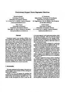
Then, a local prediction model (kernel machine) is created for each subdomain and the computations that does not depend on the test data are factored out and precomputed (e.g. inversion of matrices). The nature of the ODC generation makes these kernel machines consistent in the overlapped regions, which are the boundaries since we constraint the subdomains to be coherent. This is motivated by the notion that data lives on a manifold with local properties and consistent connections between its neighboring regions. On prediction, the output is calculated as a reduction function of the predictions on the closed subdomain(s). Table 1 ( the last row) shows the complexity for our generalized ODC framework, detailed in Sec 5.1 and 5.2. In contrast to the prior work, our ODC framework is designed to cover structured regression setting, dY > 1 and to be applicable to GPR, TGP, and many other models. Notations. Given a set of input data X = {x1 , · · · , xN }, our prediction framework firstly generates a set of non-overlapping equal-size partitions, C = {C1 , · · · , CK }, such that ∪i Ci = X, |Ci | = N/K. Then, the ODC is defined based on them as D = {D1 , · · · , DK }, such that |Di | = M ∀i, Di = Ci ∪ Oi , ∀i. Oi a the set of points that overlaps with the other partitions, i.e., Oi = {x : x ∈ {∪j6=i Cj }}, such that |Oi | = p · M , |Ci | = (1 − p) · M , 0 ≤ p ≤ 1 is the ratio of points in each overlapping subdomain, Di , that belongs to/overlaps with partitions, other than its own, Ci . It is important to note that, the ODC could be specified by two parameters, M and p, which are the number of points in each subdomain and the ratio of overlap respectively; this is since K = N/(1 − p)M . This parameterization of ODC generation is reasonable for the following reasons. First, M defines the number of points that are used to train each local kernel machine, which controls the performance of the local prediction. Second, given M and that K = N/(1 − p)M , p defines how coarse/fine the distribution of kernel machines are. It is not hard to see that as p goes to 0, the generated ODC reduces to the set of non-overlapping clusters. Similarly, as p approaches 1−1/M , the ODC reduces to generating a cluster at each point with maximum overlap with other clusters, i.e., K = N , |Ci | = 1, and |Oi | = M −1. Our main claim is two fold. First, precomputing local kernel machines (e.g. GPR, TGP, IWTGP) during training on the ODC significantly increase the speedup on prediction time. Second, given a fixed M and N , as p increases, local prediction per-

Overlapping Cover Local Regression Machines

5

Fig. 2: ODC Framework

formance increases, theoretically supported by Lemma 51 Lemma 51. Under ODC notion, as the overlap p increases, the closer the nearest model to an arbitrary test point and the more likely that model get trained on a big neighborhood of the test point. Proof. We start by outlining the main idea behind the proof, which is directly connected to the fact that K = N/(1 − p)M , which indicates that the number of local models increases as p increases given fixed N and M . Under the assumption that the local models are spatially cohesive, p → 1 theoretically indicates that there is a local model centered at each point in the space (i.e. K = ∞). Hence, as p increases, the distribution of the kernel machines is the finest and the more likely a test point to find the closest kernel machines trained on a big neighborhood of it leading to more accurate prediction. Meanwhile, as p goes to 0, the distribution is the coarsest and the less likely a test point finds, the closest kernel machines, trained on a big neighborhood. Let’s assume that each kernel machine is defined on M points that are spatially cohesive, covering the space of N N points with (1−p)M . Let’s assume that center of the M points in kernel machine i is µi , the the Co-variance matrix of these points are Σi . Hence

is an test point x∗ and define that the probability that x∗ is captured by the ODC to be proportional to the maximum probability of x∗ among the domains.

p(x∗ ) =

dX 2

=

K X

∗ p(x∗ |Di )δ(p(x∗ |Di ) − maxK j=1 (p(x |Di )))

i=1 ∗ = maxK i=1 p(x |Di )

= (2π)−

dX 2

1

1

1

T

Σi−1 (x−µi )

(5)

N N , K2 = (1 − p1 )M (1 − p2 )M

∗

−µi )T Σi−1 (x∗ −µi )

(7) where δ(0) = 1, 0 otherwise. The reason behind this definition of p(x∗ ) is that our method select the domain of preduc∗ ∗ tion based on argmaxK i=1 p(x |Di ). Hence pODC1 (x ) = K1 K2 ∗ ∗ maxi=1 pODC1 (x |Di ) and pODC2 (x ) = maxi=1 pODC2 (x∗ |Di ). We start by the case where the points are uniformally distributed in the space. Under this condition and assuming that spatially cohesive domain cover, this leads to that p(x∗ |Di ) ≈ N (µi , Σ)∀i, where Σ1 = Σ2 · · · = ΣK = Σ. Hence 1

|Σi |− 2 e− 2 (x−µi )

1

− 2 − 2 (x maxK e i=1 |Σi |

p(x∗ |Di ) ∝ e− 2 (x

where N (µi , Σi ) is a normal distribution of mean µi and Co-variance matrix Σi . Let’s assume that there are two ODCs, ODC1 and ODC2 , defined on the same N points, the first one has overlap p1 and the second one is with overlap p2 , such that, p2 > p1 . Let’s assume that the number of kernel machines in ODC1 and ODC2 are K1 and K2 , respectively. Hence, K1 =

p(x∗ , Di )

i=1

p(x|Di ) = N (µi , Σi ) = (2π)−

K X

∗

−µi )T Σ −1 (x∗ −µi )

(8)

ln(p(x∗ |Di )) ∝ −(x∗ − µi )T Σ −1 (x∗ − µi ) Then ∗ p(x∗ ) = maxK i=1 p(x |Di )

= (2π)−

dX 2

1

1

T

− 2 (x−µi ) Σ|− 2 maxK i=1 |e 1

− 2 (x−µi ) ∝ maxK i=1 e

T

Σ −1 (x−µi )

Σ −1 (x−µi )

T −1 ln(p(x∗ )) ∝ maxK (x − µi ) i=1 − (x − µi ) Σ

(9) (6)

Since p2 > p1 , 0 ≤ p1 < 1 and 0 ≤ p2 < 1, then K2 > K1 , which indicates that the number of kernel machines in ODC2 with higher overlap is bigger than the number of kernel machines in ODC2 . Let’s assume that there

Hence, p(x∗ ) gets maximized as it get closer to one of the centers of the domains µi , defined by the ODC. It is not hard to seen that that chances of x∗ to be closer to one of the centers covered by ODC2 is higher than ODC2 , especially when p2  p1 . This is since K1 = (1−pN1 )M , K2 =

6 N (1−p2 )M .

Hence K2  K1 when p2  p1 . For instance, when p1 = 0 and p2 = 0.9, this leads to that ODC1 will N domains, while ODC2 will generate generate K1 = M 10·N K2 = M = 10K1 , which is ten times more domains and centers. The fact that there are much more domains if K2  K1 together with that there domains are spatially cohesive K2 ∗ 1 T −1 ∗ 1 1 leads to maxK i=1 − (x − µi ) Σ1 (x − µi )  maxi=1 − ∗ 2 T −1 ∗ 2 (x −µi ) Σ2 (x −µi ). The proof of this statement derives ∗ T −1 ∗ from the fact that maxK (x −µi ) is could i=1 −(x −µi ) Σ ∗ maximized by (1) if x gets very close to one of µi , i = 1 : K,and (2) smaller variance |Σ|, which is minimized by the nature by which ODC is created, since each domain i is created by neighboring points to its center (i.e. |Σ1 |  |Σ2 |). ∗ 1 This directly leads to that if K2  K1 then maxK i=1 −(x − K2 1 T −1 ∗ ∗ 2 T −1 ∗ 1 µi ) Σ1 (x − µi )  maxi=1 − (x − µi ) Σ2 (x − µ2i ). Hence, pODC2 (x∗ )  pODC1 (x∗ ). Even if the points are not uniformally distributed, it is still more likely that an ODC with higher overlap would have higher p(x∗ ), since x∗ is close under expectation to one of the centers if more spatially cohesive domains are generated which increases with higher overlap. Our experiments also proves that the ODC concept generalizes on three real dataset where the training points are not distributed uniformally.

5.1 Training There are several overlapping clustering methods that include (e.g. [17] and [3]), which looks relevant for our framework. However these methods does not fit our purpose both equal-size constraints for the local kernel machines. We also found them very slow in practice because their complexity varies from cubic to quadratic (with a big constant factor) on the training-set. These problems motivated us to propose a practical method that builds overlapping local kernelmachines with spatial and equal-size constraints. These constraints are critical for our purpose since the number of points in each kernel-machine determine its local performance. Hence, our training phase is two steps: (1) the training data is split into K = N/(1 − p)M equal-sized clusters of (1 − p)M points. (2) an ODC with K overlapping subdomains is generated by augmenting each cluster with p · M points from the neighboring clusters. 5.1.1 Equal-size Clustering There are recent algorithms that deal with size constraints in clustering. For example, [29] formulated the problem of clustering with size constraints as a linear programming problem. However such algorithms are not computationally efficient, especially for large scale datasets (e.g., Human3.6M). We study two efficient ways to generate equal size clusters; see Table 1 (last row) for their ODC-complexity.

M Elhoseiny et al.

Recursive Projection Clustering (RPC) [5]. In this method, the training data is partitioned to perform GPR prediction. Initially all data points are put in one cluster. Then, two points are chosen randomly and orthogonal projection of all the data onto the line connecting them is computed. Depending on the median value of the projections, The data is then split into two equal size subsets. The same process is then applied to each cluster to generate 2l clusters after l repetitions. The iterations stops once 2l > K. As indicated, the number of clusters in this method has to be a power of two and it might produce long thin clusters. Equal-Size K-means (EKmeans). We propose a variant of k-means clustering [11] to generate equal-size clusters. The goal is to obtain disjoint partitioning of X into clusters C = {C1 , · · · , CK }, similar to the k-means objective, minimizing the within-cluster sumP of squared Euclidean distances, K P C = argC J(C) = min j=1 xi ∈Cj d(xi , µj ), where µi is the mean of cluster Ci , and d(·, ·) is the squared distance. Optimizing this objective is NP-hard and k-means iterates between the assignment and update steps as a heuristic to achieve a solution; l1 denotes number of iterations of kmeans. We add equal-size constraints ∀(1 ≤ i ≤ K), |Ci | = N/K = (1 − p)M . In order to achieve this partitioning, we propose an efficient heuristic algorithm, denoted by Assign and Balance (AB) EKmeans. It mainly modifies the assignment step of the k-means to bound the size of the resulting clusters. We first assign the points to their closest see center as typically done in the assignment step of k-means. We use C(xp ) to denote the cluster assignment of a given point xp . This results in three types of clusters: balanced, overfull, and underfull clusters. Then some of the points in the overfull clusters are redistributed to the underfull clusters by assigning each of these points to the closest underfull cluster. This is achieved by initializing a pool of overfull points defined as ˜ = {xp : xp ∈ Cl , |Cl | > N/K}; see Figure 3. X Let us denote the set of underfull clusters by C˜ = {Cp : |Cp | < N/K}. We compute the distances d(xi , µj ), ∀xi ∈ ˜ and Ci ∈ C. ˜ Iteratively, we pick the minimum distance X pair (xp , µl ) and assign xp to cluster Cl instead of cluster C(xp ). The point is then removed from the overfull pool. Once an underfull cluster becomes full it is removed from the underfull pool, once an overfull cluster is balanced, the remaining points of that cluster are removed from overfull pool. The intuition behind this algorithms is that, the cost associated with the initial optimal assignment (given the computed means) is minimally increased by each swap since we pick the minimum distance pair in each iteration. Hence the cost is kept as low as possible while balancing the clusters. We denote the the name of this Algoirthm as Assign and Balance EKmeans. Algorithm 1 illustrates the overall assignment step and Fig. 4 visualizes the balancing step.

Overlapping Cover Local Regression Machines

7

5.1.2 Overlapping Domain Cover(ODC) Model

Fig. 3: AB-EKmeans on 300,000 2D points, K= 57

Fig. 4: AB Kmeans: Balancing Step

Input: X(N × dx ), {µi }K i=1 Output: labels 1- Assign the points initially to its closest center; this will put the clusters into 3 groups (1) balanced clusters (2) overflowed clusters (3) under-flowed clusters. 2- Create a matrix D ∈ RN ×K , where D[i, j] is the distance between the ith point to the j th cluster center; rows are restricted points belongs only to the overflowed clusters; columns are restricted to underflowed cluster centers 3- Get the coordinate (i∗ , j∗ ) that maps the smallest distance in D. 4- Remove the ith ∗ row from matrix D and mark it as assigned to the j th cluster 5- If the size of the cluster j achieves the ideal size (i.e. n/K), then remove the j th column from matrix D. 6- Go to step 3 if there is still unassigned points

Algorithm 1: Assign and Balance (AB) k-means: Assignment Step

Having generated the disjoint equal size clusters, we generate the ODC subdomains based on the overlapping ratio p, such that p · M points are selected from the neighboring clusters. Let’s assume that we select only the closest r clusters to each cluster, Ci is closer to Cj than Ck if kµi − µj k < kµi − µk k. It is important to note that r must be greater than p/(1 − p) in order to supply the required p · M points; this is since number of points in each cluster is (1 − p)M . Hence, the minimum value for r is d(p · M )/((1 − p) · M )e = dp/(1 − p)e clusters. Hence, we parametrize r as r = dt · p/(1 − p)e, t ≥ 1. We study the effect of t in the experimental results section. Having computed r from p and t, each subdomain Di is then created by merging the points in the cluster Ci with p · M points, retrieved from the r neighboring clusters. Specifically, the points are selected by sorting the points in each of r clusters by the distance to µi . The number of points retrieved for each of the r neighboring clusters is inversely proportional to the distance of its center to µi . If a subset of the r clusters are requested to retrieve more than its capacity (i.e., (1 − p)M ), the set of the extra points are requested from the remaining clusters giving priority to the closer clusters (i.e., starting from the nearest neighboring cluster to the cluster on which the subdomain is created). As t = 1 and p increases, all points that belong to the r clusters tends to be merged with Ci . In our framework, we used FLANN [15] for fast NN-retrieval; see pseudo-code of ODC generation in Appendix C. After the ODC is generated, we compute the the sample normal distribution using the points that belong to each subdomain. Then, a local kernel machine is trained for each of the overlapping subdomains. We denote the point set normal distribution of the subdomains as p(x|Di ) = N (µ0i ∈ −1 RdX , Σi0 ∈ RdX ×dX ); Σ 0 i is precomputed during the training for later use during the prediction. Finally, we factor out all the computations that does not depend on the test point (for GPR, TGP, IWTGP) and store them with each sub domain as its local kernel machine. We denote the training model for subdomain i as Mi , which is computed as follows for GPR and TGP respectively. GPR. Firstly, we precompute (Kij + σn2 i I)−1 , where j

Kij is an M × M kernel matrix, defined on the input points in Di . Each dimension j in the output could have its own hyper-parameters, which results in a different kernel matrix for each dimension Kij . We also precompute (Kij +σn2 i I)−1 yj j

for each dimension. Hence MiGP R = {(Kij +σn2 i I)−1 , (Kij + j

σn2 i I)−1 yj ) , j = 1 : dY }. j

TGP. The local kernel machine for each subdomain in TGP case is defined as MiT GP = {(KiX + λiX I)−1 , (KiY + λiY I)−1 }, where KiX and KiY are M ×M kernel matrices de-

8

M Elhoseiny et al.

fined on the input points and the corresponding output points respectively, which belong to domain i. IWTGP. It is not obvious how to factor out computations that does not depend on the test data in the case of 1

i2

IWTGP, since the computational extensive factor(i.e., (W 1

1

1

KiX Wi 2 + λix I)−1 , (Wi 2 KiY Wi 2 + λiy I)−1 ) does depend on the test set since Wi is computed on test time. To help factor out the computation, we used linear algebra to show that (D A D+λI)−1 = D−1 A−1 D−1 −

λD−2 A−2 D−2 1 + λ · tr(D−1 A−1 D−1 ) (10)

where D is a diagonal matrix, I is the identity matrix, and tr(B) is the trace of matrix B. Proof. Kenneth Miller [14] proposed the following Lemma on Matrix Inverse. 1 G−1 HG−1 1 + tr(GH −1 )

(G + H)−1 = G−1 −

(11)

Applying Miller’s lemma, where G = DAD and H = λI, leads directly to Eq. 10. 1

Mapping D to Wi 2 1 , A to either of KiX or KiY , we can −1 −1 compute Mi = {KiX , KiY }. Having computed Wi on 1

1

1

1

test time, (Wi 2 KiX Wi 2 + λx I)−1 , (Wi 2 KX Wi 2 + λx I)−1 could be computed in quadratic time given Mi following 1

equation 10, since the inverse and the power of Wi 2 has linear computational complexity since it is diagonal. 5.2 Prediction ODC-Prediction is performed in three steps. (1) Finding the closest subdomains. The closest K 0  K subdomains are determined based on the covariance norm of the displacement of the test input from the means of the subdomain distribution (i.e. kx−µ0i kΣi0 −1 , i = 1 : K, where −1

kx−µ0i kΣi0 −1 = (x−µ0i )T Σi0 (x−µ0i ). The reason behind using the covariance norm is that it captures details of the density of the distribution in all dimensions. Hence, it better models p(x|Di ), indicating better prediction of x on Di . (2) Closest subdomains Prediction. Having determined the closest subdomains, predictions are made for each of the K0 closest clusters. We denote these predictions as {Yxi∗ }i=1 . Each of these prediction are computed according to the selected kernel machine. For GPR, predictive mean and variance are O(M · dX ) and O(M 2 · dY ) respectively, for each output dimension. For TGP, the prediction is O(l2 ·M 2 ·dY ); see Eq 2. 1

W is a diagonal matrix

(3) Subdomains weighting and Final prediction. The final PK 0 predictions are formulated as Y(x∗ ) = i=1 ai Yix∗ , ai > PK 0 K0 0, i=1 ai = 1. {ai }i=1 are computed as follows. Let the distribution of domain {Dxi ∗ = kx − µ0i kΣ 0 −1 } k

K0

i=1

denotes K0

to the distances to the closest subdomains, {Lix∗ = 1/Dxi ∗ }i=1 , PK 0 ai = Lix∗ / i=1 Lix∗ . It is not hard to see that when K 0 = 1, the prediction step reduces to regression using the closest subdomain to the test point. However it is reasonable in most of the prior work to make prediction using the closest model, we generalized it to K 0 closest kernel machines and combining their predictions, so as to study how consistency of the combined prediction behaves as the overlap increases (i.e., p); see the experiments.

6 Experimental Results Equal-Size Kmeans Step Experiment: We also tried another variant for Ekmeans that we call Iterative MinimumDistance Assignments EKmeans (IMDA- Ekmeans). Note that the algorithm presented earlier in the paper is denoted as Assign and Balance Kmeans (AB-Kmeans). The IMDAEkmeans algorithm works as follows. We initialize a pool ˜ = X and initialize all clusters as of unassigned points X empty. Given the means computed from the previous update steps, we compute the distances d(xi , µj ) for all points/center pairs. We iteratively pick the minimum distance pair ˜ and|Cl | < N/K (xp , µl ) : d(xp , µl ) ≤ d(xi , µj )∀xi ∈ X and assign point xp to cluster l. The point is then removed from the pool of unassigned points. if |Cl | = N/K, then it is marked as balanced and no longer considered. The process is repeated until the pool is empty; see Algorithm 2. Table 3 presents the average cost over 10 runs of IMDAEkmeans and AB-Ekmeans algorithms. We initialize both the AB-Ekmeans and IMDA-EKmeans algorithms by the cluster centers computed by running the standard k-means. Input: X(N × dx ), {µi }K i=1 Output: labels N ×K 1- Create a matrix D ∈ R , where D[i, j] is the distance between the ith point to the j th cluster center. 2- Get the coordinate (i∗ , j∗ ) that maps the smallest distance in D. 3- Remove the ith ∗ row from matrix D and mark it as assigned to the j th cluster 4- If the size of the cluster j achieves the ideal size (i.e. n/K), then remove the j th column from matrix D. 5- Go to step 2 if there is still unassigned points

Algorithm 2: Iterative Minimum-Distance Assignments (IMDA) k-means: Assignment Step

Overlapping Cover Local Regression Machines

9

As illustrated in table 3, the AB-Ekmeans outperforms IMDAEkmeans in these experiments, which motivated us to utilize AB Ekmeans, which is presented in the paper, against IMDA-Ekmeans under our ODC prediction framework. Our interpretation for these results is because AB-Ekmeans initializes the assignment with PK anPassignment that minimizes the cost J(C) = min j=1 xi ∈Cj d(xi , µj ) given the cluster centers and then balance the clusters. In all the following experiments, we uses AB-EKmeans due to its clear superior performance to IMDA-EKmeans. Table 3: J(C) of AB-kmeans and IMDA-kmeans on a dataset of 10,000 random 2D points, averaged over 10 runs

AB-kmeans IMDA-kmeans Error Reduction

K=5 1077.3 1290.6 16.53%

K = 10 540.241 657.446 17.83%

K=50 105.505 122.006 13.52%

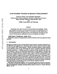
Subjects (S1, S2, S6, S7, S8, S9) from it, which is ≈ 0.5 million poses. We split them into 67% training 33% is testing. HOG features are extracted for 4 image-views for each pose and concatenated into 3060-dim vector. Error for each pose, in both HEva (in mm) and Human 3.6 (in cm), is measured 1 PL as Error(ˆ y, y∗ ) = L y m − y ∗m k. m=1 kˆ There are four control parameters in our ODC framework: M , p, t, and K 0 . Figure 6 shows our parameter analysis with different values of p, t and K 0 on HumanEva dataset for GPR and TGP as local regression machines, where M = 800. Each sub-figure consists of six plots in two rows. The first row indicates the results using AB-Ekmeans clustering scheme, while the second row shows the results for RPC clustering scheme. Each row has three plots, one for K 0 = 1, 2, and 3 respectively. Each plot shows the error of different t against p from 0 to 0.95; i.e., it shows how the overlap affects the performance for different values of t. Each plot shows, on its top caption, the minimum and the maximum overlap regression errors where t → 1. Looking at these plots, there are a number of observations: (1) As t → 1 (the solid red line), the behavior of the error tends to reduce as p increases, i.e., the overlap.

Fig. 5: Datasets, Representations, and Features

Datasets and Setup. We evaluated our framework on three human pose estimation datasets, Poser, HumanEva, and Human3.6M; see Fig. 5 for summary of setup and representation for each. Poser dataset [1] consists of 1927 training and 418 test images. The image features, corresponding to bag-of-words representation with silhouette-based shapecontext features. The error is measured by the root meansquare error (in degrees), averaged over all joints angles, and 1 P54 is given by: Error(ˆ y , y ∗ ) = 54 y m − y ∗m mod 360◦ k, m=1 kˆ 54 where yˆ ∈ R is an estimated pose vector, and y ∗ ∈ R54 is a true pose vector. HumanEva datset [20] contains synchronized multi-view video and Mocap data of 3 subjects performing multiple activities. We use HOG features [7] (∈ R270 ) proposed in [2]. We use training and validations subsets of HumanEva-I and only utilize data from 3 color cameras with a total of 9630 image-pose frames for each camera. This is consistent with experiments in [2] and [26]. We use half of the data for training and half for testing. Human3.6M [4] is a dataset of millions of Human poses. We managed to evaluate our proposed ODC-framework on six

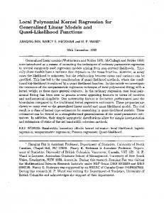
(2) Comparing different K 0 , the behavior of the error indicates that combining multiple predictions (i.e., K 0 = 2 and K 0 = 3), gives poor performance, compared with K 0 = 1, when the overlap is small. However, all of them, K 0 = 1, 2, and 3, performs well as p → 1; see column 2 and 3 in Fig. 6 and Fig. 8. This indicates consistent prediction of neighboring subdomains as p increases; see also Fig. 7 for side by side comparison of different K 0 . The main reason behind this behavior is that as p increases, the local models of the neighboring subdomains normally share more training points on their boundaries, which is reflected as shared constraints during the training of these models making them more consistent on prediction. (3) Comparing the first row to the second row in each subfigure, it is not hard to see that our AB-Ekmeans partitioning scheme consistently outperforms RPC [5], e.g. the error in cases of GPR (M=800) is 47.48mm for AB-EKmeans and 50.66mm for RPC, TGP (M=800) is 38.8mm for ABEKmeans and 39.8mm for RPC. This problem is even more severe when using smaller M , e.g. the error in case of TGP (M=400) is 39.5mm for EKmeans and 47.5mm for RPC; see a detailed plot for M=400 in Fig. 9. We noticed sigficant drop in the performance as M decreases. For instance when M = 200, The error for TGP best performance increased to 43.88mm instead of 38mm for M = 800. (4) TGP gives better prediction than GPR (i.e., 38mm using TGP compared with 47mm using GPR). (5) As M increases, the prediction error decreases. For instance, when M = 200, The error for TGP best performance increased to 43.88mm instead of 38.9mm for M = 800.

10

M Elhoseiny et al. AB EKmeans, K’ = 1, Err = [51.60,48.52]

AB EKmeans, K’ = 2, Err = [130.23,47.66]

55 54

140

160 140

t t t t t

50 49 0

= = = = =

0.2

Error

51

48

180

120

52

Error

Error

53

AB EKmeans, K’ = 3, Err = [173.13,47.49]

160

100

1.0 1.5625 2 3 4

80

0.6

0.8

40

1

100 80

60

0.4

120

60 0

0.2

0.4

p

0.6

0.8

40

1

0

0.2

0.4

0.6

p

RPC, K’ = 1, Err = [54.39,50.93]

RPC, K’ = 2, Err = [67.75,50.54]

56

0.8

1

p RPC, K’ = 3, Err = [128.13,50.67]

70

140

55

120

65

53

Error

Error

Error

54 60

100 80

52 55

60

51 50

0

0.2

0.4

0.6

0.8

50

1

0

0.2

0.4

0.6

0.8

40

1

p

p

AB EKmeans, K’ = 1, Err = [41.12,38.79]

AB EKmeans, K’ = 2, Err = [123.75,38.79]

0

0.2

0.4

0.6

0.8

1

p

(a) GPR-ODC (M=800) 42

140

41.5

120 150

40

t t t t t

39.5 39 0

0.2

= = = = =

1.0 1.5625 2 3 4

Error

100

40.5

Error

Error

41

38.5

80

100

60 50 40

0.4

0.6

0.8

20

1

0

0.2

0.4

p

0.6

0.8

0

1

RPC, K’ = 2, Err = [58.60,39.44]

60

120

55

100

41.5

Error

41 40.5

Error

140

50 45

40

0.4

0.6

0.8

1

35

0.6

0.8

1

80 60

40

39.5 0.2

0.4

RPC, K’ = 3, Err = [122.05,39.80]

65

42

0

0.2

p

42.5

39

0

p

RPC, K’ = 1, Err = [41.62,39.49]

Error

AB EKmeans, K’ = 3, Err = [166.79,38.85] 200

40

0

0.2

0.4

p

0.6

0.8

1

20

0

0.2

0.4

p

0.6

0.8

1

p

(b) TGP-ODC (M=800) Fig. 6: ODC framework Parameter Analysis of GPR and TGP on Human Eva Dataset Table 4: Error & Time on Poser and Human Eva datasets (Intel core-i7 2.6GHZ), M = 800

TGP

GPR

NN [2] ODC (p = 0.9, t = 1, K 0 = 1)-Ekmeans ODC (p = 0, t = 1, K 0 = 1)-Ekmeans ODC (p = 0.9, t = 1, K 0 = 1)-RPC ODC (p = 0, t = 1, K 0 = 1)-RPC NN ODC (p = 0.9, t = 1, K 0 = 1)-Ekmeans ODC(p = 0.0, t = 1, K 0 = 1)-Ekmeans ODC (p = 0.9, t = 1, K 0 = 1)-RPC ODC (p = 0.0, t = 1, K 0 = 1)-RPC = [5] FIC [22]

Poser Error (deg) 5.43 5.40 7.60 5.60 7.70 6.77 6.27 7.54 6.45 7.46 7.63

Training Time (3.7 +25.1 ) sec (3.9 + 1.33) sec (0.23 +41.6 ) sec (0.15 + 1.7) sec (3.7 +11.1 ) sec ( 3.9 + 1.38 sec) (0.23 +17.3 ) sec (0.15 + 1.5) sec (- + 20.63)

We found these observation to be also consistent on Poser dataset. This analysis helped us conclude recommending choosing t close to 1, big overlap (p closer to 1), and K 0 = 1 is sufficient for accurate prediction. Having accomplished the performance analysis which comprehensively interprets our parameters, we used the recommended setting to compare the performance with other methods and show the benefits of this framework. Figure 10 shows the speedup gained by retrieving the matrix inverses

Prediction Time 188.99 sec 16.5 sec 14.8 sec 15.8 sec 13.89 sec 24 sec 0.56 sec 0.35 sec 0.52 sec 0.27 sec 0.3106

HumanEva Error (mm) 38.1 38.9 41.87 39.9 42.32 54.8 49.3 49.6 52.8 54.6 68.36

Training Time (2001 + 45.4) sec (240 + 4.9 ) sec ( 0.45 + 49.1) sec (0.19 + 5.2) sec (2001 + 42.85)sec (240 + 6.4) sec (0.49 + 46.06) sec (0.26 + 4.6 ) sec -

Prediction Time 6364 sec 298 sec 257 sec 277 sec 242 sec 618 sec 79 sec 48 sec 64 sec 44 sec 102 sec

on test time, compared with computing them at test time by NN scheme. The figure shows significant speedup from precomputing local kernel machines. Table 4 shows error, training time and prediction time of NN, FIC, and different variations of ODC on Poser and Human-Eva datasets. Training time is formatted as (tc + tp ), where tc is the clustering time and tp is the remaining training time excluding clustering. As indicated in the top part of table 4, TGP under our ODC-framwork can significantly speedup the prediction compared with NN-scheme

Overlapping Cover Local Regression Machines

11

Fig. 7: HumanEva TGP different K’ as overlap increase, , M=800

Fig. 8: Increasing K’ significantly heart the performance for small overlap (Human Eva TGP, M=800)

6

10

5

Speedup

10

4

10

3

10

2

10

2

10

3

M

10

Fig. 10: Speedup of ODC framework prediction on either TGP or GPR while retrieving precomputed matrix inverses as M increases, compared with computing them on test time by KNN scheme (log-log scale)

in [2], while achieving competitive performance; better in case Poser Dataset. As illustrated in our analysis in Figure 6, higher overlap (p) gives better performance. From time analysis perspective, higher p costs more training time due that more subdomains are created and trained. While, Figure 6 and Table 4 indicates that AB-Ekmeans gives better perfor-

mance than RPC under both GPR and TGP, AB-Ekmeans takes more time for clustering. Yet, it is feasible to compute in all the datasets, we used in our experiments. Our experiments also indicate that as p → 1 in TGP and GPR, K 0 = 2 and K 0 = 3 takes double and triple the prediction time respectively, compared with K 0 = 1, with almost no error reduction. We also compared our model to FIC in case of GPR, and our model achieved smaller error and smaller prediction time; see bottom part in Table 4. However, TGP consistently gives better results on both Poser and HumanEva datasets. We also tried full TGP and GPR on Poser and Human Eva Datasets. Full TGP error is 5.35 for Poser and 40.3 for Human Eva. Full GPR error is 6.10 for Poser and 59.62 for Human Eva. The results indicate that ODC achieves either better or competitive to the full models. Meanwhie, the speedup is sigbificant for TGP prediction (21X for Human Eva and 11X for Poser Datasets); see Fig. 11. For GPR prediction, we achieved the best performance and the lowest prediction time compared to existing GPR prediction methods; see Fig. 12. Based on our comprehensive experiments on HumanEva and Poser datasets, we conducted an experiment on Human3.6M dataset with TGP kernel machine, where M = 1390, t = 1, p = 0.6, K 0 = 1, Ekmeans for clustering. We achieved a speedup of 41.7X on prediction time using our ODC framework compared with NN-scheme, i.e., 7 days if NN-scheme is used versus 4.03 hours in our case with our MATLAB implementation. The error is 13.5 (cm) for NN and 13.8 (cm) for ODC; see Fig. 13. 7 Conclusion We proposed an efficient ODC framework for kernel machines and validated the framework on structured regression machines on three human pose estimation datasets. The key idea is to equally partition the data and create cohesive overlapping subdomains, where local kernel machines are computed for each of them. The framework is general and could be applied to various kernel machine beyond GPR, TGP, IWTGP validated in this work. Similar to TGP and IWTGP,

12

M Elhoseiny et al.

Fig. 11: TGP Human Eva Dataset (Speed)

Fig. 12: GPR speed and error (Human Eva Dataset)

Fig. 13: TGP speed and error (Human3.6M Dataset)

our framework could be easily applied to the recently proposed Generalized TGP [8] which is based on Sharma Mittal divergence, a relative entropy measure brought from Physics community. We also theoretically justified our framework’s notion. Acknowledgment. This research was partially funded by NSF award # 1409683.

References 1. Agarwal, A., Triggs, B.: Recovering 3d human pose from monocular images. PAMI (2006) 2. Bo, L., Sminchisescu, C.: Twin gaussian processes for structured prediction. Int. J. Comput. Vision 87(1-2), 28–52 (2010) 3. Bonchi, F., Gionis, A., Ukkonen, A.: Overlapping correlation clustering. Knowledge and information systems 35(1), 1–32 (2013) 4. Catalin Ionescu Dragos Papava, V.O., Sminchisescu, C.: Human3.6M: Large Scale Datasets and Predictive Methods for 3D Human Sensing in Natural Environments. Tech. rep., nstitute of Mathematics at the Romanian Academy and University of Bonn (2012)

5. Chalupka, K., Williams, C.K.I., Murray, I.: A framework for evaluating approximation methods for gaussian process regression. JMLR 14(1) (2013) 6. Cristianini N. Shawe-Taylor, J., Kandola, J.S.: Spectral kernel methods for clustering. In: NIPS (2001) 7. Dalal, N., Triggs, B.: Histograms of oriented gradients for human detection. In: CVPR, vol. 1, pp. 886 –893 vol. 1 (2005). DOI 10.1109/CVPR.2005.177 8. Elhoseiny, M., Elgammal, A.: Generalized twin gaussian processes using sharma-mittal divergence. Machine Learning pp. 1– 26 (2015) 9. Gramacy, R.B., Lee, H.K.H.: Bayesian treed gaussian process models with an application to computer modeling. Journal of the American Statistical Association (2007) 10. Gretton, A., Bousquet, O., Smola, A., Sch¨olkopf, B.: Measuring statistical dependence with hilbert-schmidt norms. In: International conference on Algorithmic Learning Theory (2005) 11. Hartigan, J.A., Wong, M.A.: Algorithm as 136: A k-means clustering algorithm. J. Roy. Statist. Soc. Ser. C) (1979) 12. Hoerl, A.E., Kennard, R.W.: Ridge Regression: Biased Estimation for Nonorthogonal Problems. Technometrics (1970) 13. Khandekar, R., Kortsarz, G., Mirrokni, V.: On the advantage of overlapping clusters for minimizing conductance. Algorithmica 69(4), 844–863 (2014) 14. Miller, K.S.: On the inverse of the sum of matrices. Mathematics Magazine 54(2), 67–72 (1981) 15. Muja, M., Lowe, D.: Fast approximate nearest neighbors with automatic algorithm configuration. In: VISAPP, pp. 331–340 (2009) 16. Park, C., Huang, J.Z., Ding, Y.: Domain decomposition approach for fast gaussian process regression of large spatial data sets. Journal of Machine Learning Research 12, 1697–1728 (2011) 17. P´erez-Su´arez, A., Mart´ınez-Trinidad, J.F., Carrasco-Ochoa, J.A., Medina-Pagola, J.E.: Oclustr: A new graph-based algorithm for overlapping clustering. Neurocomputing 121, 234–247 (2013) 18. Rasmussen, C.E., Williams, C.K.I.: Gaussian Processes for Machine Learning (Adaptive Computation and Machine Learning). The MIT Press (2005) 19. Seeger, M.: Fast forward selection to speed up sparse gaussian process regression. In: in Workshop on AI and Statistics 9 (2003) 20. Sigal, L., Balan, A.O., Black, M.J.: Humaneva: Synchronized video and motion capture dataset and baseline algorithm for evaluation of articulated human motion 21. Snelson, E.: Local and global sparse gaussian process approximations. In: AISTATS (2007) 22. Snelson, E., Ghahramani, Z.: Sparse gaussian processes using pseudo-inputs. In: NIPS (2006) 23. Tresp, V.: A bayesian committee machine. NEURAL COMPUTATION 12, 2000 (2000) 24. Urtasun, R., Darrell, T.: Sparse probabilistic regression for activity-independent human pose inference. In: CVPR (2008) 25. Williams, C., Seeger, M.: Using the nystrm method to speed up kernel machines. In: NIPS (2001) 26. Yamada, M., Sigal, L., Raptis, M.: No bias left behind: covariate shift adaptation for discriminative 3d pose estimation. In: ECCV (2012) 27. Yamada, M., Suzuki, T., Kanamori, T., Hachiya, H., Sugiyama, M.: Relative density-ratio estimation for robust distribution comparison. In: NIPS, pp. 594–602 (2011) 28. Yuksel, S., Wilson, J., Gader, P.: Twenty years of mixture of experts. Neural Networks and Learning Systems, IEEE Transactions on (2012) 29. Zhu, S., Wang, D., Li, T.: Data clustering with size constraints. Knowledge-Based Systems 23(8), 883 – 889 (2010)

13

Appendices A IWTGP-ODC Experiments Tables 5 and 6 details the results of IWTGP-ODC experiments on Poser and HumanEva datasets in terms of error and speedup in prediction time.

error (deg) err reduction (deg) err reduction % Prediction Time (sec) speedUp

IWTTGP (M = 800, Mtst = 418) 6.1 360.0 -

IWTGP-ODC (M = 800, Mtst = 418) 5.32 0.783 12.836% 26.61 13.5

Table 5: POSER dataset IWTGP-NN vs IWTGP-ODC

error (mm) err reduction (mm) err reduction % Prediction Time (sec) speedUp

IWTGP (M = Mtst = 800)

IWTTGP-ODC (M = Mtst = 800)

39.1 7938.15 -

39.3 -0.2 -0.512% 569.66 13.92

(a) 5 clusters Fig. 14: Applying our Assign and Balance variant of Kmeans on 300,000 random 2D points

Table 6: Humen Eva dataset: IWTGPKNN vs IWTGP-ODC

B More figures on AB Ekmeans Figure 14 shows the clustering performance on 300000 random 2D point (K=5). Figure 15 shows the clustering output of our algorithm visualized on using the first three principal components of Human Eva training hog features. The figures shows that the cluster are spatially cohesive but not necessarily circular. This makes the elliptic distribution of the data captured by Mode 3 gives more accuracy membership measure me to the subdomains.

Fig. 15: Human Eva clustering first three Pricipal Components

ested in. The following subsection present the learnt hyperparameters and the error measures on each dataset in case of TGPs.

C Overlapping Domain Cover(ODC) Generation-Algorithm D.1 Poser Dataset Algorithm 3 shows how the overlapping sub-domains are generated form the the equal size clusters from the closest r clusters.

The parameters 2ρ2x , 2ρ2y , λX , and λY were assigned to 5, 5000, 10−4 , and 10−4 , respectively.

D Local Kernel Machines hyper-parameters on each dataset

D.2 HumanEva Dataset

The hyper parameters were learnt using cross validation on the training set for GPR, TGP and IWTGP that we are inter-

The parameters 2ρ2x , 2ρ2y , λX , and λY were assigned to 5, 500000, 10−3 , and 10−3 , respectively.

14 Input: Clusters {Ck }K k=1 Output: Overlapping subdomains {Dk }K k=1 foreach Cluster Ck do 0 r Compute the closest r clusters {C i }i=1 based on DKi = kµk − µi k , i 6= k i i=1:r Let LKi = 1/DKi , W Ki = POLK CC l=1

LKl

Let N P Ki = f loor(W Ki ∗ OP P C), i = 1 : r Let ExKP ts = (1 − p)M − rl=1 N P Kl Let N P Ki = N P Ki + 1 , i = 1 : ExKP ts D k = Ck Let overf low = 0 . The following for loop goes over the r clusters on an increasing order of DKi for i=1 : r do if N P Ki ¿ |Ci | then overf low = overf low + N P Ki − |Ci | N P Ki = |Ci | if N P Ki ¡ |Ci | then Gi = min(overf low, |Ci | − N P Ki ) N P K i = N P K i + Gi overf low = overf low − Gi P si = KN N (OV CK j , N P Ki ) Dk = Dk ∪ P si for i=1 : r do P si = KN N (OV CK j , N P Ki ) Dk = Dk ∪ P si . where KNN is the K-nearest neighbors algorithms. For high performance calculation of KN N , we use FLANN [15] to calculate KN N .

Algorithm 3: Subdomains Generation (Note: All K {Dk }k=1 are stored as indices to X). D.3 Human 3.6 Dataset The parameters 2ρ2x , 2ρ2y , λX , and λY were assigned to 5, 500000, 10−3 , and 10−3 , respectively.

15 AB EKmeans, K’ = 1, Err = [41.53,39.23]

AB EKmeans, K’ = 2, Err = [52.95,39.13]

42

AB EKmeans, K’ = 3, Err = [122.62,39.51]

100

140

41.5

120 80

t t t t t

40 39.5 0

0.2

1.0 1.5625 2 3 4

60

80 60

40 40

0.4

0.6

0.8

20

1

0

0.2

0.4

0.6

0.8

20

1

0

0.2

0.4

0.6

0.8

p

p

p

RPC, K’ = 1, Err = [41.77,40.40]

RPC, K’ = 2, Err = [107.41,41.73]

RPC, K’ = 3, Err = [136.14,47.45]

42.5

160

42

140

1

200

150

41

Error

120

41.5

Error

Error

39

= = = = =

Error

100

40.5

Error

Error

41

100

100

80 50

40.5

60

40

40

0

0.2

0.4

0.6

0.8

1

0

0.2

0.4

p

0.6

0.8

0

1

0

0.2

0.4

p

0.6

0.8

1

p

(a) TGP-ODC (M=400) AB EKmeans, K’ = 2, Err = [81.89,45.35]

AB EKmeans, K’ = 3, Err = [147.56,45.29]

100

160

51

90

140

50

80

120

49

t t t t t

48 47 46

0

0.2

= = = = =

1.0 1.5625 2 3 4 0.4

0.6

0.8

70

100

60

80

50

60

40

1

Error

52

Error

Error

AB EKmeans, K’ = 1, Err = [50.24,46.51]

0

0.2

0.4

0.6

0.8

40

1

0

0.2

0.4

0.6

0.8

p

p

p

RPC, K’ = 1, Err = [54.01,50.96]

RPC, K’ = 2, Err = [112.22,49.86]

RPC, K’ = 3, Err = [156.13,50.56]

55

120

1

160 140

54

100

52

Error

Error

Error

120 53

80

100 80

60

51 50

60 0

0.2

0.4

0.6

p

0.8

1

40

0

0.2

0.4

0.6

0.8

p

1

40

0

0.2

0.4

0.6

0.8

1

p

(b) GPR-ODC (M=400) Fig. 9: Overlapping Domain Cover Parameter Analysis of GPR and TGP on Human Eva Dataset (best seen in color) (M=400)

16

Mohamed Elhoseiny is a PostDoc Researcher at Facebook Research. His primary research interest is in computer vision, machine learning, intersection between natural language and vision, language guided visual-perception, and visual reasoning, art & AI. He received his PhD degree from Rutgers University, New Brunswick, in 2016 under Prof. Ahmed Elgammal. Mohamed received an NSF Fellowship in 2014 for the Write-aClassifier project (ICCV13), best intern award at SRI International 2014, and the Doctoral Consortium award at CVPR 2016. Ahmed Elgammal is a professor at the Department of Computer Science, Rutgers, the State University of New Jersey Since Fall 2002. Dr. Elgammal is also a member of the Center for Computational Biomedicine Imaging and Modeling (CBIM). His primary research interest is computer vision and machine learning. His research focus includes human activity recognition, human motion analysis, tracking, human identification, and statistical methods for computer vision. Dr. Elgammal received the National Science Foundation CAREER Award in 2006. Dr. Elgammal has been the Principal Investigator and Co-Principal Investigator of several research projects in the areas of Human Motion Analysis, Gait Analysis, Tracking, Facial Expression Analysis and Scene Modeling; funded by NSF and ONR. Dr. Elgammal is Member of the review committee/board in several of the top conferences and journals in the computer vision field. Dr. Elgammal received his Ph.D. in 2002 from the University of Maryland, College Park. He is a senior IEEE member.