A VARIATIONAL MODEL FOR SEGMENTATION OF OVERLAPPING OBJECTS WITH ADDITIVE INTENSITY VALUE YAN NEI LAW∗ , HWEE KUAN LEE∗ , CHAOQIANG LIU† , AND ANDY M. YIP‡ Abstract. We propose a variant of the Mumford-Shah model for the segmentation of overlapping objects with additive intensity value. Unlike standard segmentation models, it does not only determine distinct objects in the image, but also recover possibly multiple membership of the pixels. To accomplish this, some a priori knowledge about the smoothness of the objects is taken into account in the model. To solve the optimization problem involving geometric quantities efficiently, we apply a multi-phase level set method. Segmentation results on synthetic and real images validate the good performance of our model. Key words. Image segmentation, Euler’s elastica, level set methods, Mumford-Shah segmentation model, additive model, overlapping objects. AMS subject classifications. 68U10, 65K10
1. Introduction. We consider the problem of segmenting two overlapping objects whose intensity level in the intersection is approximately the sum of the level of the individual objects. Mathematically speaking, assume that O1 and O2 are two possibly overlapping objects in a domain Ω. We consider images u0 : Ω → R which can be well modeled by the following piecewise constant function u : Ω → R: c1 , if (x, y) ∈ O1 \ O2 , c2 , if (x, y) ∈ O2 \ O1 , u(x, y) = c + c , if (x, y) ∈ O1 ∩ O2 , 1 2 c3 , if (x, y) ∈ Ω \ (O1 ∪ O2 ). We shall call the identification of O1 and O2 from a given image u0 as an additive segmentation problem. This is a fundamental image processing task with many real world applications especially those involving measurement of concentration using imaging techniques. Examples include x-ray images, images of absorbent paper with mouse scent marks [7], and microscopy images recording protein expression [6]. Although many applications of such a model can be found, there has been little study of this problem. Many types of segmentation have been studied. They include hard segmentation [5, 11], soft segmentation [4, 15], segmentation with depth [12, 13, 19], illusory object segmentation [18], and segmentation of touching objects [17]. Additive segmentation fundamentally differs from other segmentation problems in two aspects — multiple membership and additivity. Except for soft segmentation, all the aforementioned ∗ Imaging Informatics Group, Bioinformatics Institute, A*STAR, 30 Biopolis Street, #07-01 Matrix, Singapore 138671. Email: {lawyn,leehk}@bii.a-star.edu.sg. This work was supported (in part) by the Biomedical Research Council of A*STAR (Agency for Science, Technology and Research), Singapore. † Centre for Wavelets, Approximation and Information Processing, National University of Singapore, 2, Science Drive 2, Singapore 117543, Singapore. Email:
[email protected]. Research supported by the Wavelets and Information Processing Programme under a grant from DSTA, Singapore. ‡ Department of Mathematics, National University of Singapore, 2, Science Drive 2, Singapore 117543, Singapore. Email:
[email protected]. Questions, comments, or corrections to this document may be directed to this email address. Research supported in part by National University of Singapore under the grants R-146-050-079-101 and R-146-050-079-133.
1
2
Y.N. Law, H.K. Lee, C. Liu and A.M. Yip
segmentation problems do not allow multiple membership of the pixels. For soft segmentation, each pixel is given a degree of membership to various objects, but the additivity of intensity values is not considered. Standard segmentation models aim at grouping pixels with similar characteristics together to determine distinct objects in the image. However, in additive segmentation, the characteristics (e.g. intensity levels) of the overlapped region are very different from that of the individual objects. Thus an additive segmentation model requires to group pixels with different characteristics together. As we will illustrate in Fig. 2.1, this requires us to consider not only the intensity value, but also the geometry of the objects. To accomplish this, we assume certain smoothness of the objects. We found that Euler’s elastica is particularly effective. In this paper, we propose a variational model for additive segmentation. We analyze a hard constrained and a soft constrained version of the model. We demonstrate that the soft one is more robust and practical. We also present a numerical scheme based on a multi-phase level set method. Segmentation results on synthetic and real images validate the good performance of our model. 2. Model. Our model is a variant of the piecewise constant Mumford-Shah segmentation model [11] which uses a least squares approach to fit the image with a piecewise constant function and uses a penalty method to regularize the geometry of the partition. However, instead of using length regularization as in the original Mumford-Shah model, we use Euler’s elastica which is more effective in recovering multiple membership. We also study the effectiveness of a hard constrained and a soft constrained way to model additivity through a simple but illustrative example. 2.1. Mumford-Shah Segmentation Model. The Mumford-Shah segmentation model [11] is one of the most popular segmentation models. It can handle gracefully complex situations and is very robust to noise. A distinctive feature is that it is region-based which allows it to segment objects without edges. For the same reason, it can group a cluster of smaller objects into a larger object. For a given image u0 , the piecewise constant Mumford-Shah model seeks for a set of curves C and a set of constants c = (c1 , c2 , . . . , cn ) which minimize the following energy functional: F
MS
(C, c) =
n Z X i=1
|u0 (x, y) − ci |2 dxdy + α × Length(C).
(2.1)
Ωi
The curves in C partition the image into n mutually exclusive segments Ωi for i = 1, 2, . . . , n. The idea is to partition the image so that the intensity of u0 in each segment Ωi is well-approximated by a constant ci . The goodness-of-fit is measured R by the fidelity term Ωi |u0 (x, y) − ci |2 dxdy. A minimum description length principle is employed to regularize the geometry of the partition. This increases the robustness to noise and avoids spurious segments. The parameter α > 0 controls the trade-off between the goodness-of-fit and the length of the curves C. It can be easily shown that for each fixed C, the optimal constant ci is given by the average of u0 over Ωi . 2.2. Euler’s Elastica. To motivate Euler’s elastica, consider the example shown in Fig. 2.1. The original image u0 consists of two crossing objects O1 and O2 with the same intensity value and the intensity of their common part is the sum. Consider the four possible segmentations in Fig. 2.1(b). All of them are consistent with the additive assumption. However, we would like to make the a priori assumption that objects
Additive segmentation of overlapping objects
3
Original image
(a) Configuration 1 Configuration 2 Configuration 3 Configuration 4
1
2
(b) Fig. 2.1. An example of two crossing objects. (a) Original image. (b) Four different segmentations which are consistent with the additivity assumption. Configuration 1 has the smallest Euler’s elastica energy.
with smooth boundaries are preferred. In this case, Configuration 1 is preferred. To achieve this, we consider the notion of Euler’s elastica [10, 9, 1, 2]. A curve Γ is said to be Euler’s elastica if it is the equilibrium curve of the elasticity energy Z E(Γ) = (α + β|κ|)ds, Γ
where ds is the arc length element, κ(s) is the scalar curvature of Γ, and α and β are two non-negative constants controlling the weighting of the length and the total absolute curvature terms. It can be seen that Configuration 1 has the minimal Euler’s elastica energy. We note that the length regularization in the Mumford-Shah model corresponds to setting β = 0. In this case, the length of Configurations 1, 2 and 3 are identical so that Configuration 1 cannot be distinguished from the others. The use of total absolute curvature can resolve this problem. In our implementation, we use Z E(Γ) = (α + βφ(κ))ds, Γ
where ½ φ(x) =
x2 , |x|,
if |x| ≤ 1, if |x| > 1.
This modification can preserve high curvature features such as corners better.
4
Y.N. Law, H.K. Lee, C. Liu and A.M. Yip
2.3. A Hard Additive Model. We start off by stating some assumptions of the additive segmentation problem. 1. There is no self-overlapping — the overlapping region must be generated by two distinct objects. 2. Intensity within each object can be well-approximated by a binary image. 3. Objects are preferred to have smooth boundary. Given an image u0 , we seek for two regions Ω1 , Ω2 and a set of constants c = (c1 , c2 , c3 , c4 ) which minimize the following energy: Z 2 Z X (u0 (x, y) − c3 )2 dxdy F hard (Ω1 , Ω2 , c) = [α + βφ(κ)]ds + i=1
Z
∂Ωi ∩Ω
Ω\(Ω1 ∪Ω2 )
Z
2
+
(u0 (x, y) − c2 )2 dxdy
(u0 (x, y) − c1 ) dxdy + Ω1 \Ω2
Ω2 \Ω1
Z
(u0 (x, y) − c4 )2 dxdy,
+ Ω1 ∩Ω2
subject to an additivity constraint c4 = c1 + c2 . This model enforces strict additivity in the overlapping region and therefore we refer it as the hard additive model. Although Ω1 and Ω2 generally do not constitute a partition of Ω, we still call the pair {Ω1 , Ω2 } a segmentation of Ω for simplicity. It should be clear that the partition of Ω is given by {Ω1 \ Ω2 , Ω2 \ Ω1 , Ω1 ∩ Ω2 , Ω \ (Ω1 ∪ Ω2 )}. Given a fixed segmentation {Ω1 , Ω2 }, it can be easily shown that the optimal constants c are given by the following formulas: ¸ · ¸ · ¸−1 · R u dxdy c1 |Ω1 | |Ω1 ∩ Ω2 | Ω1 0 R , = · u dxdy c2 |Ω1 ∩ Ω2 | |Ω2 | Ω2 0 R u dxdy Ω\(Ω1 ∪Ω2 ) 0 c3 = . (2.2) |Ω \ (Ω1 ∪ Ω2 )| Here, | · | denotes the Lebesgue measure of its argument. The above linear system is non-singular if and only if neither of the objects is empty and Ω1 6= Ω2 . In many applications, the additivity assumption may not be exactly satisfied. In this case, due to the possible ill-conditioning of the above linear system, the resulting constants c1 and c2 may be totally different from the observed intensity values even for a small deviation in additivity in the overlapping region. According to some numerical tests of the hard additive model, we observe that the natural approach of level set method often converges to a bad local minimum, cf. Section 4.1 for an example. Hence, we attempt to solve this problem by relaxing the hard constraint to a soft one. 2.4. A Soft Additive Model. We consider the following relaxed model: Z 2 Z X soft [α + βφ(κ)]ds + (u0 (x, y) − c3 )2 dxdy F (Ω1 , Ω2 , c) = i=1
Z
∂Ωi ∩Ω
Ω\(Ω1 ∪Ω2 )
Z
(u0 (x, y) − c1 )2 dxdy +
+ Ω1 \Ω2
(u0 (x, y) − c2 )2 dxdy Ω2 \Ω1
Z
2
(u0 (x, y) − c4 ) dxdy + γ(c1 + c2 − c4 )2 ,
+ Ω1 ∩Ω2
5
Additive segmentation of overlapping objects Area = ε
O1\O2 u0=d1
O1∩O2 u0=d1+d2
Area = ε
1∩
O2\O1 u0=d2
\(O1∪O2) u0=d3
1\
\(
(a)
1∪
2 2\
2
1
2)
(b)
Fig. 2.2. (a) Two objects O1 and O2 with constant intensity level d1 and d2 overlapping each other. (b) The dashed (resp. solid) curve represents the boundary of the initial segmentation Ω1 (resp. Ω2 ) with a perturbation of size ².
where γ ≥ 0 is a constant controlling the additivity. In this model, the constraint c1 + c2 = c4 is only loosely enforced. We call this model the soft additive model. Note that when γ = 0, the soft model reduces to the piecewise constant MumfordShah segmentation model [11, 16]. When γ → ∞, the solution of the soft model will approach to that of the hard model. Given a segmentation {Ω1 , Ω2 }, the optimal constants c = (c1 , c2 , c3 , c4 ) can be obtained by the following explicit formulas:
c1 |Ω1 \ Ω2 | + γ γ c2 = γ |Ω2 \ Ω1 | + γ c4 −γ −γ R u dxdy Ω\(Ω1 ∪Ω2 ) 0 . c3 = |Ω \ (Ω1 ∪ Ω2 )|
−1 R u dxdy 0 −γ Ω \Ω R 1 2 · −γ R Ω2 \Ω1 u0 dxdy , |Ω1 ∩ Ω2 | + γ u0 dxdy Ω ∩Ω 1
2
(2.3)
When γ > 0, this linear system is non-singular if and only if neither of the objects is empty and Ω1 6= Ω2 . 2.5. Analysis of the Hard and Soft Additive Models. In this subsection, we analyze the robustness of F hard and F soft with respect to different parameters through some simple but illustrative examples. In these examples, we can see how the key ingredients — the constants c — affect the solution of both models in practice. The results below can be derived by directly comparing for each pixel the differences between each of the constants (c1 , c2 , c3 , c4 ) and the intensity level of the pixel. Example 1: Perturbation analysis. Here we study the energy change of the fidelity term (i.e., when α = β = 0) in F hard and F soft when the initial segmentation is a controlled perturbation of the ideal segmentation. Consider an image u0 with two objects O1 and O2 shown in Fig. 2.2(a). Fig. 2.2(b) shows an initial segmentation Ω1 (dashed curve) and Ω2 (solid curve). We assume that Oi ⊂ Ωi ⊂ O1 ∪ O2 ,
for i = 1, 2,
6
Y.N. Law, H.K. Lee, C. Liu and A.M. Yip
and
d1 , d2 , u0 (x, y) = d 1 + d2 , 0,
if if if if
(x, y) ∈ O1 \ O2 , (x, y) ∈ O2 \ O1 , (x, y) ∈ O1 ∩ O2 , (x, y) ∈ Ω \ (O1 ∪ O2 ).
Let A1 = |O1 \ O2 |,
A2 = |O2 \ O1 |,
A12 = |O1 ∩ O2 |,
² = |Ω1 \ O1 | = |Ω2 \ O2 |.
Thus ² is the area of the perturbation of O1 and O2 . We assume that ² < min{A1 , A2 }. Except for Ω1 \ O1 and Ω2 \ O2 , we shall assume that all the aforementioned regions are non-empty. Each pixel in the initial segmentation takes one of the four states: Ω1 \Ω2 , Ω2 \Ω1 , Ω1 ∩ Ω2 and Ω \ (Ω1 ∪ Ω2 ). We study the energy change when each pixel changes its state from one to another. In particular, we focus on two kinds of state transition: 1) complete transition and 2) gray-code transition which are illustrated in Fig. 2.3(a) and (b) respectively. The former transition is natural to consider while the latter transition is implicitly used in the level set method presented in the next section. 1\
1∩
(
2
1∪
2\
2
(a)
2)’
1
1\
1∩
(
2
1∪
2\
2
2)’
1
(b)
Fig. 2.3. Two kinds of state transitions: (a) Complete transition and (b) Gray-code transition.
Let F = F (Ω1 , Ω2 , c) be an energy function (F = F hard or F = F soft in this paper). Given a segmentation {Ω1 , Ω2 }, we study one pass of the following steps to update the segmentation: ˜ using Eq. (2.2) or Eq. (2.3) with the 1. Compute the optimal constants c segmentation fixed at {Ω1 , Ω2 }; 2. For each pixel in Ω, change its state to a neighboring state in the transition graph G such that the energy F is minimized with respect to the state of the pixel while the state of other pixels is fixed at its value in {Ω1 , Ω2 } and the ˜, i.e. Jacobi-type update. constants are fixed at c We shall call this procedure one sweep of steepest descent of F with respect to the state transition graph G. We remark that we consider Ω1 and Ω2 as functions of ². ˜ 1, Ω ˜ 2 } are also functions of ². ˜ and the new segmentation {Ω Thus, the new constants c In order to draw simple and concrete conclusions, we fix d1 = 105, d2 = 130, A1 = A2 = 2198, A12 = 611 and 0 < ² < min{A1 , A2 } in the sequel. Note that we do not specify the area of the background since it does not affect the value of (c1 , c2 , c4 ) and the decision of the state transitions. Starting with the segmentation in Fig. 2.2(b), six segmentations are possible, depending on the specification of ², F and G. These segmentations are depicted in Fig. 2.4.
7
Additive segmentation of overlapping objects 2
1
2
Segmentation 3
Segmentation 6
Segmentation 2
Segmentation 5
Segmentation 4
Segmentation 1
1
Fig. 2.4. Six possible segmentations after one sweep of steepest descent is taken.
Observation 2.1. The result of one sweep of steepest descent of F hard with α = β = 0 and with complete state transition is given by: Segmentation 1, if ² ∈ [0, 217), ˜ 1, Ω ˜ 2} = Segmentation 2, if ² ∈ [217, 921), {Ω Segmentation 3, if ² ∈ [921, 2198). The result of one sweep of steepest descent of F hard with α = β = 0 and with gray-code state transition is given by: ½ Segmentation 1, if ² ∈ [0, 921), ˜ ˜ {Ω1 , Ω2 } = Segmentation 4, if ² ∈ [921, 2198). We observe that for a large value of ², the steepest descent will lead to an unsatisfactory segmentation. Next, we demonstrate that the soft additive model F soft can lead to a better result. Indeed, we derive an upper bound of γ in terms of the perturbation ² below which the soft model can resolve the above issue. Observation 2.2. For each ² ≥ 0, there is an upper bound γ0 such that one sweep of steepest descent of F soft with α = β = 0, γ < γ0 and with both complete and gray-code state transitions will lead to the ideal segmentation {O1 , O2 }. Indeed the wrong assignment of O1 \ O2 to Ω2 \ Ω1 (which exists in Segmentations 2 and 3 in Fig. 2.4) will be corrected if γ < γ1 (²) :=
5(2198 − ²)2 (611 + 2²) , 94(2198 − ²)² − 5(7517160 + 3174² − 3²2 )
while the wrong assignment of O2 \ O1 to Ω1 ∩ Ω2 (which exists in Segmentations 3 and 4 in Fig. 2.4) will be corrected if γ < γ2 (²) :=
105(2198 − ²)(611 + ²) − 130²(2198 − ²) . 6594² − 359100
Thus, when complete transition is used (where Segmentations 1, 2 and 3 are possible), the upper bound is given by γ0 (²) = min{γ1 (²), γ2 (²)}.
(2.4)
8
Y.N. Law, H.K. Lee, C. Liu and A.M. Yip
When gray-code transition is used (where Segmentations 1 and 4 are possible), the upper bound is given by γ0 (²) = γ2 (²).
(2.5)
3000
3000
2500
2500
2000
2000
1500
1500
γ0
γ0
The upper bound γ0 under complete and gray-code state transitions are shown in Fig. 2.5(a) and (b) respectively. We observe that the smaller the ², the larger the range of γ is available. Hence, for each ² < min{A1 , A2 }, the soft model with a suitable choice of γ will lead to the ideal solution. We remark γ = 0 always leads to the ideal segmentation in this example. But in practice we would like to choose γ as large as possible to ensure additivity.
1000
1000
500
500
0 0
500
1000 ε
1500
2000
0 0
500
(a)
1000 ε
1500
2000
(b)
Fig. 2.5. (a) γ0 vs. ² under complete state transition, cf. Eq. (2.4). (b) γ0 vs. ² under gray-code state transition, cf. Eq. (2.5).
Example 2: Deviation in additivity in the overlapping region. In this example, we study the case when the additivity assumption is not exactly satisfied. Consider again the image in Fig. 2.2(a), but with the intensity level in the overlapping region changed to σ(d1 + d2 ) where σ > 0. When σ 6= 1, the additivity is not exact. In particular, we are only interested in the case when the intensity of the overlapping region is larger than the intensity of the two objects and smaller than the maximum allowable intensity dmax (e.g. 255 for an 8-bit image), i.e., max(d1 , d2 ) dmax 0, = 0, ψi (x, y) < 0,
if (x, y) ∈ Ωi , if (x, y) ∈ ∂Ωi , if (x, y) ∈ Ω \ Ωi .
Then, the proposed soft additive energy functional can be reformulated as F soft (ψ1 , ψ2 , c) =
2 Z X
[α + βφ(κi )]|∇ψi |δ(ψi )dxdy
i=1
Ω
+
(u0 (x, y) − c1 )2 H(ψ1 )[1 − H(ψ2 )]dxdy
Z ZΩ
(u0 (x, y) − c2 )2 [1 − H(ψ1 )]H(ψ2 )dxdy
+ Z
Ω
Z
Ω
(u0 (x, y) − c3 )2 [1 − H(ψ1 )][1 − H(ψ2 )]dxdy
+
(u0 (x, y) − c4 )2 H(ψ1 )H(ψ2 )dxdy
+ Ω
+γ|c1 + c2 − c4 |2 . ∇ψi where κi = ∇ · ( |∇ψ ) and H : R → R is the Heaviside function defined by i|
1, 1 , H(x) = 2 0,
if x > 0, if x = 0, if x < 0.
3.2. Level Set Based Gradient Descent Method. To optimize the functional F soft (Ψ, c), we use an alternating minimization approach where the objective is minimized with respect to Ψ and c alternatively. Using standard variational calcu-
Additive segmentation of overlapping objects
11
lus, the gradient flow for F soft (·, c) can be derived as ½ ¾ ∂ψi ∇ψi 1 0 = |∇ψi |∇ · [α + βφ(κi )] − (I − P ∇ψi )∇ [βφ (κi )|∇ψi |] |∇ψi | ∂t |∇ψi | |∇ψi | © ª 2 2 − |∇ψi | [(u0 − ci ) − (u0 − c3 ) ][1 − H(ψj )] + [(u0 − c4 )2 − (u0 − cj )2 ]H(ψj ) (3.1) for i = 1, 2 and j = 3 − i, see [19]. Here, I is the identity operator and Pn : R2 → R2 is the projector defined by Pn (v) = (v · n)n for v ∈ R2 . The boundary condition is ∂ψi ∂n = 0 on ∂Ω. This system of equations is solved numerically by standard explicit finite difference methods. The detailed numerical implementation can be found in [19]. The gradient flow for F hard (·, c) is almost the same. We only need to replace c4 by c1 + c2 in Eq. (3.1). When we update the constants c, Eq. (2.2) is used instead of Eq. (2.3). 4. Numerical Results. We validate our model based on 1) several performance comparisons with some competitive methods; 2) the robustness to different parameters; 3) the applicability to diverse applications. 4.1. Comparison of various models. Hard vs. Soft Models. In this test, we experiment the analysis in Section 2.5. We compare the hard and the soft models with α = β = 0 using the image in Fig. 2.2. The objective is optimized using the level set method introduced in Section 3. The intensity of the two objects are d1 = 105 and d2 = 130 respectively. The area (number of pixels) of various regions are |O1 \ O2 | = |O2 \ O1 | = 2198 and |O1 ∩ O2 | = 611. The results of minimizing F hard with the level set algorithm are shown in Fig. 4.2. According to the result of Observation 2.1, the range of area perturbation within which a sweep of steepest descent of F hard will lead to a wrong solution is given by ² ∈ [921, 2198). In this example, we have ² = 1022. We observe that the level set algorithm also results in the same wrong solution as the steepest descent algorithm, cf. Observation 2.1. The use of the soft model will lead to the correct segmentation, see Fig. 4.3. Mumford-Shah Model vs. Soft Model. In this test, we use an image containing two irregular shapes with intensity value 70 and 180. The intensity value in their overlapping region is 250. The original image and the initial segmentation are shown in the first row of Fig. 4.4. The results in the second row show that in this experiment the proposed method is able to segment out the two objects successfully even if the initial condition is far away from the exact segmentation. Next we compare the performance of the soft model with the four-phase MumfordShah segmentation model. The latter model corresponds to setting β = γ = 0 in the soft model. The result of the four-phase method is shown in the third row. As expected, the four-phase method alone is not sufficient to correctly segment images with overlapping objects. Indeed the iterates are trapped in a local minimum. For example, in the segment Ω2 , there are three small isolated pieces. Shrinking these pieces will reduce the total length of Ω2 and keep the fitting term unchanged. Unfortunately, the total length of Ω1 may increase so that the segmentation is reluctant to change. However, when the soft model is used, the fitting term may be reduced by shrinking the small spurious pieces.
12
Y.N. Law, H.K. Lee, C. Liu and A.M. Yip
Original image
Initial
Initial
1
2
Fig. 4.1. Original image and initial segmentation.
Intermediate segmentation
Intermediate
Final segmentation
Final
1
Intermediate
Final
1
2
2
Fig. 4.2. Intermediate and final segmentation results obtained by the hard additive model.
Intermediate segmentation
Intermediate
Final segmentation
Final
1
1
Intermediate
Final
2
2
Fig. 4.3. Intermediate and final segmentation results obtained by the soft additive model.
4.2. Robustness to different parameters. In this experiment, we show that the soft model is robust to initial guess, deviation in additivity, and inhomogeneity of intensity. Robustness to initial guess. The original image and the initial segmentation are shown in the first row of Fig. 4.5. The intensity value of the two objects and the overlapping region are 70, 180 and 250 respectively. We use a ‘seed’ initial condition, which is a commonly used generic condition. In the image, the two objects cross over each other so that the non-overlapping region of each object becomes disconnected. This adds some difficulty to the identification of the correct segmentation since many
13
Additive segmentation of overlapping objects
Initial
1
Initial
2
Final segmentation
Final
1
Final
2
Final segmentation
Final
1
Final
2
Mumford-Shah model
Soft model
Original image
Fig. 4.4. Results of the soft additive model and the four-phase Mumford-Shah model. 1st row: Original image with size 128 × 128 and the initial segmentation. 2nd row: Soft additive model with α = 1000, β = 0, and γ = 5000. 3rd row: Four-phase Mumford-Shah model with α = 1000 and β = γ = 0.
connections are possible. Thus it invokes the use of some smooth connectivity assumptions. The results in the second row show that the proposed method is able to segment out the two objects successfully. Robustness to deviation in additivity. In this test, we use again the image in Fig. 4.5 except the intensity value of the objects are now 100 and 130. The intensity value of the overlapping region is varied (i.e. σ(100+130) with a varying σ). We apply the hard model and the soft model with α = β = 0 using level set implementations. We use the ideal segmentation as the initial segmentation. By using an analysis similar to the one in the Observation 2.3, we deduce that the ideal segmentation is not a fixed point of F hard with respect to pixel-wise perturbation when σ < 0.65. For each σ ∈ {0.60, 0.61, 0.62, 0.63, 0.64, 0.65}, we minimize F soft with different γ’s using the level set approach and empirically determine the cut-off value γ0 below which the method stabilizes at the ideal segmentation. Such empirical results are compared against the analytical estimate in Observation 2.4 in Fig. 4.6. The two sets of results agree very well with each other. In particular, when minimizing F hard , the level set approach encounters a similar problem as with the steepest descent approach discussed in Observation 2.3. The problem may be resolved by minimizing F soft instead. Robustness to inhomogeneity of intensity. In this test, we use a real x-ray image to demonstrate how our method works in real world scenarios. The original image and a manual segmentation are shown in the first row of Fig. 4.7. The image exhibits a certain degree of additivity but the intensity level within each region is
14
Y.N. Law, H.K. Lee, C. Liu and A.M. Yip
Original image
Initial
1
Initial
2
Final segmentation
Final
1
Final
2
Fig. 4.5. Segmentation result on the synthetic crossing marks image. 1st row: Original image with size 100 × 100 and the initial condition of two level set functions. 2nd row: Soft additive model with α = 100, β = 50 and γ = 1000.
Parameter γ0
800
Empirical Analytical
600
400
200
0 0.6
0.61
0.62 0.63 Variation σ
0.64
0.65
Fig. 4.6. Comparison of the analytically and empirically determined cut-off values γ0 as a function of the deviation σ. The analytical results, derived for the steepest descent algorithm, parallel to the results in Section 2.5. The empirical results are obtained using the level set approach with α = β = 0.
highly inhomogeneous. The intensity distribution of each segment is summarized below: mean pelvis 60.6094 34.5987 femur overlap 106.4818 background 3.3792
standard deviation 37.3692 15.9237 22.4055 7.6219
Note that the intensity of the overlapping region is almost the same as the sum of the intensities of the femur and pelvis. The second row of Fig. 4.7 shows the initial segmentation used. The results in the third row show that the proposed soft model is able to obtain a fairly good segmentation. The pelvis is captured correctly. The femur
15
Additive segmentation of overlapping objects
Original image background
Manual
1
Manual
2
overlap
pelvis
femur
Initial segmentation
Initial
1
Initial
2
Final segmentation
Final
1
Final
2
Fig. 4.7. Segmentation results of the hip joint image. 1st row: Original image with size 240 × 240 and the initial segmentation. 2nd row: Results of the soft additive model with α = 2200, β = 10 and γ = 1000.
is slightly off. We note that the intensity of the pelvis near the top left corner is as bright as the overlapping part which makes the image difficult to segment correctly. As a result, the method assigns this corner as part of the overlapping region. 4.3. Other applications. To further illustrate the usefulness of the proposed model, we apply it to two other applications: density-based clustering and colored imaging. Density-based clustering. In this test, we use a binary image to represent a data set consisting of two dimensional data points. The intensity of a pixel is 255 if it is populated with at least one point and 0 otherwise. The data set contains two overlapping clusters. We assume that each cluster is of approximately uniform density and that the density is additive at where clusters overlap. Here, the density R 1 of a region R may be taken as |R| u dxdy. The task is to find the clusters. The 0 R original image and the initial segmentation are shown in the first row of Fig. 4.8. Note that this task is different from the aforementioned additive segmentation in that the intensity levels are no longer additive in the present case. It is the density which is additive. Indeed, the intensity levels within a cluster are far from uniform so that the fidelity term is not even close to 0. But our method can segment the two clusters effectively. The results are shown in the second row of Fig. 4.8.
16
Y.N. Law, H.K. Lee, C. Liu and A.M. Yip
Original image
Initial
1
Initial
2
Final segmentation
Final
1
Final
2
Fig. 4.8. Segmentation results of the image representing a 2-D data set. 1st row: Original image with size 100 × 100 and the initial segmentation. 2nd row: Results of the soft additive model with α = 10000, β = 0 and γ = 10000.
Multi-channel images. In this test, we use a multi-channel microscopy image of a cell nucleus which captures the p53 and mdm2 protein concentration profiles in the green and red channels respectively. The task is to segment two colored overlapping objects. The aforementioned (single-channel) soft additive model can be easily generalized to handle multi-channel images. The generalized model is as follows: F
soft
(Ω1 , Ω2 , c) =
2 Z X i=1
Z
Z ku0 (x, y) − c3 k2 dxdy
[α + βφ(κ)]ds + ∂Ωi ∩Ω
Ω\(Ω1 ∪Ω2 )
Z
ku0 (x, y) − c1 k2 dxdy +
+ Z
Ω1 \Ω2
ku0 (x, y) − c2 k2 dxdy Ω2 \Ω1
ku0 (x, y) − c4 k2 dxdy + γkc1 + c2 − c4 k2 .
+ Ω1 ∩Ω2
Here u0 : Ω → Rm is the observed multi-channel image and ci ∈ Rm for i = 1, 2, 3, 4 are constant vectors. The results are depicted in Fig. 4.9. In the second row, the boundary of the objects is overlaid on the top of each channel. Since the signals from red and green channels are quite well-separated, the ground truth of each channel can be easily obtained for comparison. The results show that the soft model is able to separate the two proteins and the background accurately. 5. Discussion. In this paper, we propose a variational model for the segmentation of overlapping objects with additive intensity value. Unlike standard segmentation models, a successful additive segmentation model needs to recover possibly multiple membership of the pixels. We achieve this by modeling additivity explicitly and incorporating geometric prior using Euler’s elastica. We also show that the soft additive model is more robust than the hard model with respect to deviation of additivity and global convergence. We remark that we use gradient descent and level set implementation to optimize the objective because of their simplicity. Our focus is the modeling aspect, leaving the computational procedure not optimized for speed. But one can readily replace
17
Additive segmentation of overlapping objects
Original image
Final segmentation
Initial
1 in
1
green-channel
Initial
2 in
2
red-channel
Fig. 4.9. Segmentation results of the microscopy image. 1st row: Original image with size 92 × 73 and the initial segmentation. 2nd row: The boundary of the objects obtained by the soft additive model with α = 100, β = 0, and γ = 1000, overlaid in the color image (left), green channel image (center) and red channel image(right).
the optimization procedure by any faster alternatives. Moreover, as with any local optimization method, the result depends very much on the initial condition. We alleviate this problem by choosing some good initial conditions. However, global optimization algorithms can be used, see, for example, [8]. As the first attempt to solving additive segmentation problems, we identified some fundamental difficulties even for the case of two objects. Future work should consider the segmentation of multiple objects and non-constant intensity objects. REFERENCES [1] T. Chan, S.H. Kang, and J. Shen, Euler’s elastica and curvature based inpaintings, SIAM J. Appl. Math., 63 (2002), pp. 564–592. [2] Tony F. Chan, Selim Esedoglu, and Mila Nikolova, Algorithms for finding global minimizers of denoising and segmentation models, SIAM J. Appl. Math., 66 (2006), pp. 1632–1648. [3] Tony F. Chan and Luminita A. Vese, Active contours without edges, IEEE Trans. Image Process., 10 (2001), pp. 266–277. ¨l Rousson, and Rachid Deriche, A review of statistical approaches [4] Daniel Cremers, Mikae to level set segmentation: Integrating color, texture, motion and shape, International Journal of Computer Vision, 72 (2007), pp. 195–215. ˜ oz, D. Raba, Joan Mart´ı, and Xavier Cuf´ı, Yet another [5] Jordi Freixenet, Xavier Mun survey on image segmentation: Region and boundary information integration, Lecture Notes in Comp. Sci., Proc. of ECCV ’02(III), 2352 (2002), pp. 408–422. [6] N. Geva-Zatorsky, N. Rosenfeld, S. Itzkovitz, R. Milo, E. Sigal, A. Dekel, T. Yarnitzky, P. Liron, Y. Polak, G. Lahav, and U. Alon, Oscillations and variability in the p53 system, Molecular Systems Biology, 2 (2006). [7] J.L. Hurst, Scent marking and social communication, Cambridge University Press, Cambridge, 2005, pp. 219–243.
18
Y.N. Law, H.K. Lee, C. Liu and A.M. Yip
[8] Y.N. Law, H.K. Lee, and A. Yip, A multi-resolution stochastic level set method for MumfordShah image segmentation, IEEE Trans. Image Process., accepted for publication (2008). [9] A. Masnou and J.-M. Morel, Level-lines based disocclusion, in Proc. of 5th IEEE Int’l Conf. on Image Process., vol. 3, 1998, pp. 259–263. [10] D. Mumford, Elastica and computer vision, Algebraic Geometry and its Applications, (1994), pp. 491–506. [11] D. Mumford and J. Shah, Optimal approximation by piecewise smooth functions and associated variational problems, Comm. Pure Appl. Math., 42 (1989), pp. 577–685. [12] M. Nitzberg and D. Mumford, The 2.1d sketch, in Proc. of the 3rd Intl. Conf. on Computer Vision, 1990, pp. 138–144. [13] M. Nitzberg, D. Mumford, and T. Shiota, Filtering, segmentation, and depth, SpringerVerlag New York, Inc., Secaucus, NJ, USA, 1993. [14] S. Osher and J. A. Sethian, Fronts propogating with curvature-dependent speed: Algorithms based on Hamilton-Jacobi formulation, J. Comput. Phys., 79 (1988), pp. 12–49. [15] J. Shen, A stochastic-variational model for soft Mumford-Shah segmentation, International Journal of Biomedical Imaging, 2006, Article ID 92329 (2006). [16] Luminita A. Vese and Tony F. Chan, A multiphase level set framework for image segmentation using the Mumford and Shah model, International Journal of Computer Vision, 50 (2002), pp. 271–293. [17] P. Yan, X. Zhou, and S. Wong, Automatic segmentation of high-throughput RNAi fluorescent cellular images, IEEE Trans. Info. Tech. Biomed., 12 (2008), pp. 109–117. [18] W. Zhu, Variational models for illusory contours and shape prior segmentation, PhD thesis, Dept. of Math., UCLA, 2005. ¯ lu, Segmentation with depth: a level set approach, SIAM [19] W. Zhu, T. Chan, and S. Esedog J. Sci. Comput., 28 (2006), pp. 1957–1973.